the Creative Commons Attribution 4.0 License.
the Creative Commons Attribution 4.0 License.
 | 28 Sep 2021
Virtual mapping and analytical data integration: a teaching module using Precambrian crystalline basement in Colorado's Front Range (USA)
Michael G. Frothingham
Ellen Alexander
The COVID-19 pandemic hindered the ability to conduct field geology courses in a hands-on and boots-on traditional manner. In response, we designed a multi-part virtual field module that encompasses many of the basic requirements of an advanced field exercise, including designing a mapping strategy, collecting and processing field observations, synthesizing data from field-based and laboratory analyses, and communicating the results to a broad audience. For the mapping exercise, which is set in deformed Proterozoic crystalline basement exposed in the Front Range of Colorado (USA), student groups make daily navigational decisions and choose stations based on topographic maps, Google Earth satellite imagery, and iterative geological reasoning. For each station, students receive outcrop descriptions, measurements, and photographs from which they input field data and create geologic maps using StraboSpot. Building on the mapping exercise, student groups then choose from six supplements, including advanced field structure, microstructure, metamorphic petrology, and several geochronological datasets. Because scientific projects rarely end when the mapping is complete, the students are challenged to see how samples and analytical data may commonly be collected and integrated with field observations to produce a more holistic understanding of the geological history of the field area. While a virtual course cannot replace the actual field experience, modules like the one shared here can successfully address, or even improve on, some of the key learning objectives that are common to field-based capstone experiences while also fostering a more accessible and inclusive learning environment for all students.
- Article
(12783 KB) - Full-text XML
-
Supplement
(43151 KB) - BibTeX
- EndNote


The COVID-19 pandemic hindered our ability to conduct in-person field geology courses and prompted worldwide efforts to design effective alternative online educational experiences. We designed an activity that can be delivered remotely and conducted virtually while still providing an effective learning experience centered on field mapping skills. We also wanted to create a capstone experience that challenges students to go beyond creating a map and understanding the basic three-dimensionality of geologic structures but also to gain a deeper appreciation for how scientific endeavors are commonly conducted through subsequent laboratory analyses and integration of the results with field-based relationships.
Field mapping exercises have traditionally been a central component of undergraduate geology curricula. Historically, development of field geology skills was integral to students' preparation for entry into the geoscience workforce (Heath, 2003; Whitmeyer et al., 2009b). Recent educational research has additionally identified benefits of field work across multiple disciplines, including improved student motivation and learning outcomes relative to traditional classroom-based education (Stokes and Boyle, 2009; Fedesco et al., 2020). The 2021 report from the Future of Undergraduate Geoscience Education initiative (Mosher and Keane, 2021) found that collaborative, problem-based learning exercises – typical of both virtual and in-person field activities – not only improve overall learning outcomes, but also are specifically beneficial for inclusion and retention of students from historically underrepresented minority groups. Virtual field exercises provide similar educational benefits with enhanced accessibility (Stokes et al., 2019) and decreased cost of participation relative to in-person field work (Abeyta et al., 2021). Furthermore, with rapid improvement and evolution in digital mapping and online collaboration tools (Walker et al., 2019), integrating modern technology into education is a valuable addition to virtual and traditional in-person field courses (Whitmeyer et al., 2009a).
In this contribution, we describe a multi-part activity involving virtual mapping and group collaboration with associated analytical datasets (Fig. 1). Part I is a mapping exercise that simulates doing field work in the Front Range of Colorado (USA) while creating a geologic map and cross section of deformed igneous and metamorphic rocks (Fig. 2). Part II introduces additional analytical datasets (e.g., microstructure, petrology, and geochronology) from the same field area, which students incorporate into their study of the area's geological history. For Part III, students produce a final report and present their results to the class. The activity is designed for an upper-level undergraduate field course for geology majors. As a remotely taught module, this activity is not intended to introduce basic field skills or outcrop-level interpretation but rather to facilitate integration and synthesis of multiple data types and develop holistic geologic interpretation skills. Students should have already been introduced to basic field methods and an introductory structural geology course. Ideally, students will have also had at least one of the following additional courses of introductory earth materials, mineralogy, petrology, or geochemistry, but the activities may be modified in such a way that those prerequisites may not be necessary. The module should take approximately 2 weeks to complete in an immersive field course (all day, every day) or could be spread over a longer period during a semester.
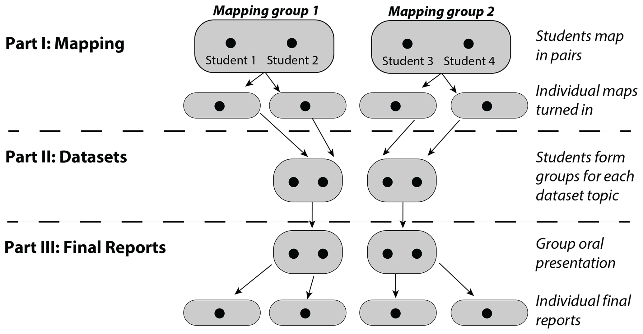
Figure 1Schematic flowchart illustrating the multi-part structure of the module and emphasizing the combination of group and individual activities. See the text for further description.

Figure 2(a) Map of exposed Proterozoic rocks in the southwestern United States with major provinces and shear zones (modified after Karlstrom and Williams, 2006). FM–LM: Farwell Mountain–Lester Mountain zone. (b) Simplified geological map of Proterozoic exposures in the Front Range (modified after Tweto, 1979). Colorado Mineral Belt boundaries in both (a) and (b) approximated from Tweto and Sims (1963), Chapin (2012), and Caine et al. (2010).
2.1 Learning objectives
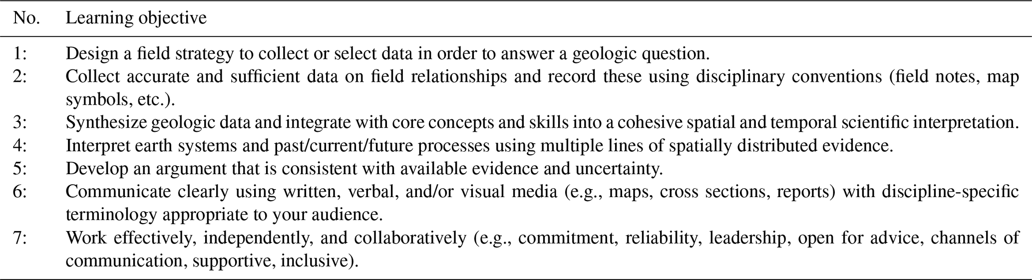
Participants in the 2020 Designing Remote Field Experiences project (Atchison et al., 2021) developed a flexible set of learning objectives to which most capstone field courses can target (whether delivered remotely or in person). This module is designed to address a subset of those objectives (Table 1). Here, we briefly describe the mechanisms for each objective.
Table 1Learning objectives.
The Designing Remote Field Experiences project was sponsored by the National Association for Geoscience Teachers and International Association for Geoscience Diversity and the National Science Foundation.
For Objective 1, student groups (e.g., mapping partners) select a fixed number of stations for each of the “field mapping days” and justify their requests based on considerations of safety, access, exposure, and geological reasoning. For Objective 2, students compile map data from outcrop descriptions of each station that include information such as rock types, features, fabrics, structures, measurements, photos, and sketches for each selected station. Objectives 3 and 4 are addressed by interpreting map relations using fundamental geological principles during each virtual mapping day as well as integrating the results from additional dataset analysis during Part II. For Objective 5, students develop multiple working hypotheses throughout their mapping, design data acquisition strategies to efficiently test those hypotheses, identify uncertainty from station description data, and project this uncertainty (e.g., certain vs. approximate contacts) into their preferred mapping interpretations that best fit the available evidence. The combination of outcrop interpretation and laboratory analytical data requires students to grapple with a range of types of uncertainty, some of which are quantifiable in a straightforward manner and some of which are not. For Objective 6, this module strengthens modern communication skills by encouraging the use of video-conferencing tools with screen sharing for collaborative work, interactive learning, and professional presentations, each of which pairs well with digital technology for mapping and quantitative analysis. Addressing Objective 7, students participate in this module through a combination of whole-class discussions, individual assignments, small group collaborative mapping, small group drop-in meetings, and small group oral presentations to the entire class.
2.2 Materials provided
Module materials are listed in Table 2, described in the Appendix and provided in the Supplement (Mahan et al., 2021b). They can also be accessed from the Teach the Earth activities portal hosted by the Science Education Resource Center (SERC) at Carleton College (Mahan et al., 2021a). Materials are provided with substantial detail to provide context for instructors and project scaffolding for students. Instructors are encouraged to modify or adapt the materials and their delivery to customize this module for various course needs. For the Part I mapping exercise, the minimum required materials are the station descriptions. Additional resources include introductory materials, instructional documents, data request forms, station location shapefiles, base maps, and other resources to aid instructors and students throughout the module (Appendix A1). For the Part II analytical data integration, students may have variable prior exposure to geochemistry, geochronology, petrology, and structural geology course work. Therefore, a set of instructional resources was assembled to provide the requisite background knowledge to conduct such analyses. These resources are a combination of published materials (journal articles and datasets), handouts, and assignments created for each of the six datasets (Appendix A2). The assignment documents enumerate the data's source publication(s) and additional files or resources as well as dataset-specific learning objectives, suggested figures to create, and questions to answer for the final report and presentation (Part III). These assignments are provided as editable Word documents that can be customized as desired. For Part III, an example set of instructional guidance and a grading rubric are also provided for the written report (Appendix A3).

2.3 Technology requirements and recommendations
During the COVID-19 pandemic, most students and instructors participated in this module from their homes using personal computers and the Internet. Thus, we designed the activities and materials such that all necessary software is either free or commonly accessible through university or college resources. Part I mapping uses Google Earth and StraboSpot software (Walker et al., 2019). StraboSpot is an integrated mapping, field data collection, and data management and storage tool and is the primary software tool for this project. StraboSpot streamlines importing station shapefiles, interactive collaboration within mapping groups, and integration of digital mapping into final figures and deliverables. The Google Earth Web project seamlessly integrates station locations and oriented viewpoint photographs with satellite imagery and 3-D topography to assist students in visualizing and selecting station locations. The web applications of both programs can perform all functions necessary for the project without the need to individually install software or download associated datasets. Alternatively, the StraboSpot mobile application also runs on tablets and mobile phones, and it provides additional offline mapping capabilities if desired. The detailed StraboSpot setup instructions are optimized for the web version.
Part II analyses require a variety of web or desktop software, depending on the dataset and analytical technique. Most datasets require spreadsheet software (e.g., Microsoft Excel or Google Sheets), advanced structural analysis also requires free stereonet software such as Stereonet 11 (Cardozo and Allmendinger, 2013; Allmendinger et al., 2013) or Orient (Vollmer, 2015), and microstructural analysis requires either the freeware MTEX toolbox (Bachmann et al., 2010; Hielscher and Schaeben, 2008) for MATLAB or the commercial Channel 5 software from Oxford Instruments.
The field area is in the Front Range of Colorado (USA), and it hosts poly-deformed intrusive and supracrustal crystalline rocks (Fig. 2). The basic map-scale structures include a kilometer-scale synform of Coal Creek quartzite and schist structurally overlying Boulder Creek granodiorite, with one limb overprinted by the Idaho Springs–Ralston shear zone (Taylor, 1976; Widmann et al., 2000; Kellogg et al., 2008). Outcrop-scale fabrics and structures include relict bedding and multiple generations of foliation and schistosity, open to isoclinal folds with axial planar foliation, mylonitic foliation, mineral and stretching lineations, and locally well-developed shear sense indicators.
The diverse geologic history of Colorado's Front Range, spanning ca. 1.8 billion years, offers several avenues to attract students' interests and effectively motivate them to learn (e.g., Stokes and Boyle, 2009). Two potential perspectives on the region may provide such motivation: (1) the features that illuminate how this part of Laurentia was built during Paleoproterozoic time and (2) their possible relations to subsequent deformation and economic mineralization. First, the exposed rocks and structures in this field area reflect the processes that formed Colorado's Proterozoic continental crust, including island-arc magmatism, back-arc basin sedimentation and inversion, low- to medium-pressure and high-temperature regional metamorphism, and polyphase deformation (e.g., Whitmeyer and Karlstrom, 2007; Jones et al., 2009). We recommend providing students with a short paper to read at the beginning of this module to introduce some of these concepts in Colorado without directly addressing the targeted map area. The paired geological and seismic study of a terrane boundary in northernmost Colorado by Tyson et al. (2002) is a good example. Second, the map area lies along the trend of the Colorado Mineral Belt (Fig. 2, which includes Cenozoic intrusions and associated mineral deposits (e.g., gold, silver, molybdenum) that have played a major role in Colorado's socioeconomic development over the last 200 years (Chapin, 2012). Tweto and Sims (1963) suggested a Proterozoic ancestry for the belt based on a series of similarly oriented (NE-striking) ductile shear zones, one of which occurs in the map area (i.e., Idaho Springs–Ralston shear zone) and another of which is described by Tyson et al. (2002). Whether or not there is a connection between these Cenozoic features and the older Proterozoic structures is still debated (e.g., Caine et al., 2010; McCoy et al., 2005).
At the University of Colorado, we run this module as a three-part virtual field course. These include an introduction, Part I, mapping, Part II, additional analytical datasets, and Part III, final reports and presentations. We begin with introductory lectures and warm-up activities such as ones that introduce concepts of field data uncertainty (e.g., Tikoff, 2020a), brief introductions to StraboSpot (e.g., Tikoff, 2020b; Walker et al., 2019), and mapping in relatively simple geologic terrain (e.g., Houghton et al., 2015; Houghton, 2020). These serve to (re-)familiarize students with key concepts and tools that they need for the mapping exercise and to help overcome initial concerns or barriers to engagement (e.g., Stokes and Boyle, 2009; Orion and Hofstein, 1994). Additionally, warm-up assignments may illuminate an individual student's strengths and weaknesses in order to assign complementary mapping partners for the following Part I exercise.
4.1 Part I: mapping
The mapping exercise is the foundation of this module. This component should take approximately 4 d if the course is taught full time, similar to a traditional field-camp module. However, if run during the semester, when students are also taking other courses, each “mapping day” can be spread over a number of actual days. Students map in pairs to encourage teamwork but also to simulate real field work in which collaborative decision-making skills are required for planning and safety. To simulate a typical day of “field” mapping, we developed a “daily” mapping schedule and describe it here in five steps: (1) introduction, (2) route planning and station selection, (3) mapping, (4) drop-in meetings, and (5) continued mapping. Each step is briefly described below.
We typically begin each mapping day with a regularly scheduled class meeting. For the first day, this may be used to introduce the field area (see “Geologic background”), goals for the mapping exercise, software, and logistics. Subsequent meetings are used to introduce more advanced geological concepts, discuss mapping strategies, and address student questions. Appendix A1 includes resources that may help introduce the field area through several different approaches. For example, the Powerpoint slides introduce the main map units and some common lithological and structural features. The Google Earth Web project may be used to interactively explore satellite imagery, topography, station locations, and oriented photographs from the field area (Fig. 3). Additionally, the class may visit some key mapping stations together in order to demonstrate and practice collecting “field data” from outcrop descriptions. Some station descriptions include quite a lot of information, requiring students to recognize the most relevant data to collect for mapping, and some guidance from instructors may be helpful here.
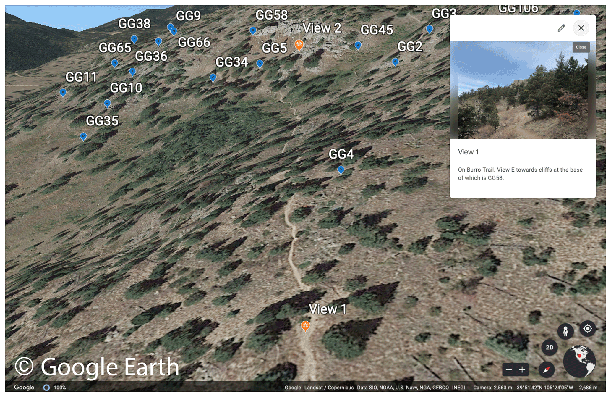
Figure 3View of the field area from one of the vantage points provided in the Google Earth Web project.
The next step is for each student group to select their mapping stations for the day. We consider about 15 stations per day to be reasonable given the terrain and common degree of complexity encountered at outcrops. Students can use the Google Earth Web project or other resources to plan their route using logistical considerations (e.g., safety, access, exposure) and geological reasoning. Before receiving station descriptions, students build a strategy for each “mapping day” by completing and submitting a station description request and justification form. The form requires students to list the selected stations, describe the route to access them, and calculate logistics such as round trip distance, time, and elevation change. This encourages students to use diverse rationales to choose their specific stations, as they would in the field, instead of choosing random or consecutively numbered stations. The form also includes specific prompts to explain how their planned strategy will test specific working hypotheses (based on previous mapping days), promoting iterative scientific reasoning that builds with each mapping day. By the end of the 4 mapping days, each group will likely have selected different combinations of 60 stations (out of 110) using varied strategies for their final maps, yet the class as a whole should have encountered most of the rocks, fabrics, and structures across the field area.
The third step is for students to begin mapping. This includes various tasks, such as setting up the basemap, extracting relevant outcrop data from station descriptions, and depicting those data on a map. We intend this module to use StraboSpot as a data management and mapping platform. Instructions for setting up the basemap with spot locations (Fig. 5) and populating them with data are described in Appendix A1 and the Supplement. If accessibility prevents digital mapping, students can instead print and use a paper basemap (Appendix A1). However, StraboSpot offers some helpful digital mapping capabilities that are not achievable with paper methods, especially when including multiple attributes for each spot.
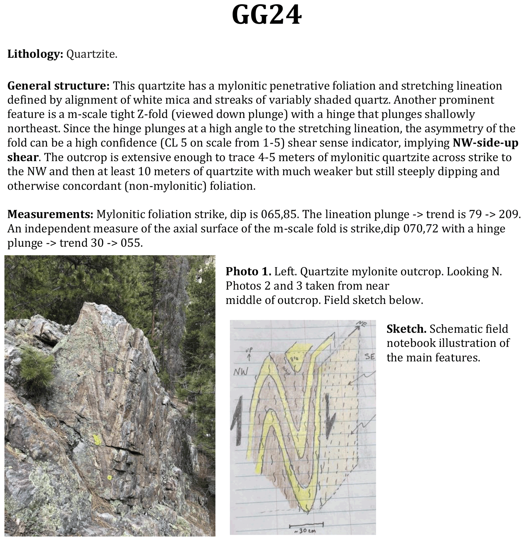
Figure 4Part of a typical outcrop description.
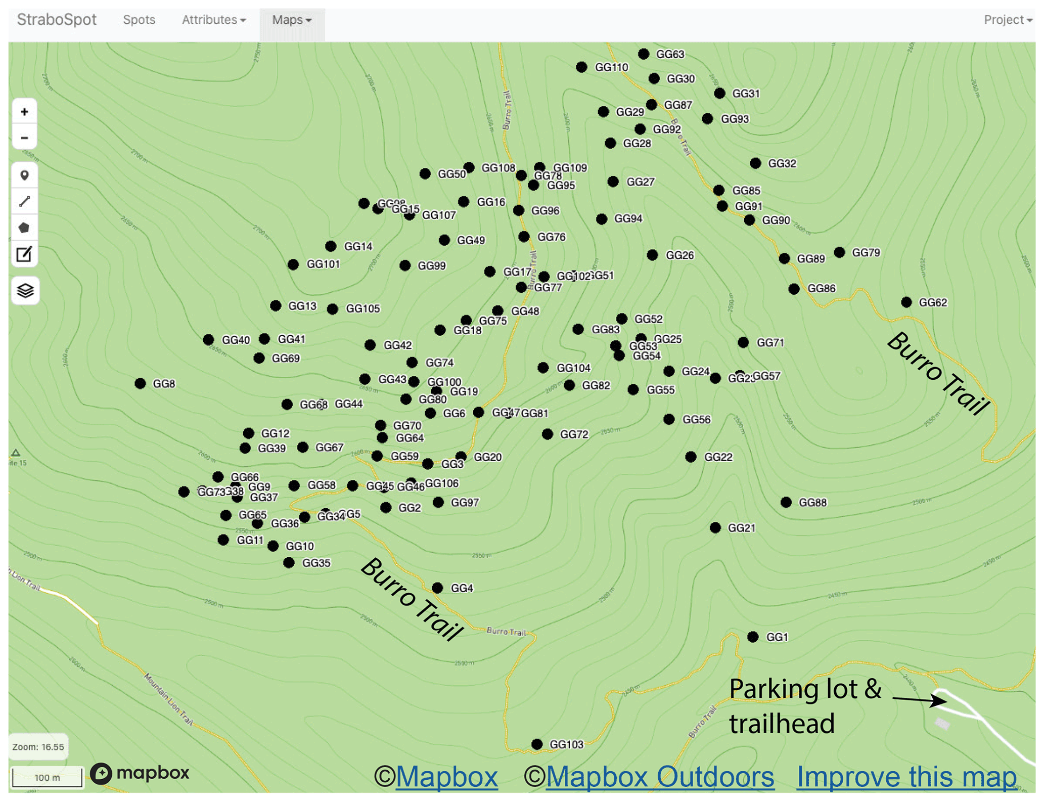
Figure 5Map view from within a StraboSpot project where the initial shapefile with outcrop locations has been imported. Labels for the parking lot and trails added in larger font for clarity.
The next task in the third step is to read, filter, and extract relevant outcrop data from each station description (Fig. 4). StraboSpot allows each spot to host various types of data, such as bedding, foliation, and lineation measurements for point spots, contact certainty, or fault type for line spots as well as rock type for polygon spots. We initially encourage students to copy and paste the text description of the outcrop information in its entirety into the “Notes” section of a spot – simply because it streamlines the process of going back to review ones notes later. Students must then decide which aspects of this description, or what specific data, are most important for mapping and working out field relationships, and using standard structural notation and terminology for relative ages (e.g., Sect. 13.2 in Fossen, 2016). For example, in some outcrops, multiple orientation measurements may be provided, but perhaps only one that could be considered “representative” is necessary for entering into the specific orientation section of the spot so that a strike and dip symbol can be displayed on the map. Or, as another example, some outcrops display conglomeratic horizons in the quartzite – this may not seem important to a student initially, but later they might decide that they want to go back to the descriptions and “tag” those outcrops with conglomeratic horizons for display on the map. Satellite imagery and topography may also complement outcrop information. Students then use fundamental geologic principles to interpolate between mapping stations and across the entire field area, while developing multiple working hypotheses to explain map relations.
The fourth step is for an instructor to remotely “drop in” on student groups. In this regularly scheduled meeting, students screen share their current work (e.g., map) and observations with their group partner(s) and the instructor, describe their working hypotheses and plans to test them, ask questions and receive feedback. This mimics the concept of instructors episodically joining a mapping team on the outcrops in the field. Two major advantages of these drop-in meetings are the abilities to interact during real-time mapping and decision-making and to digitally annotate on each other's shared screens and maps. At the end of this meeting, the instructor moves on to another group while leaving the students to continue mapping on their own.
Step five involves continued mapping with the rest of that day's stations, refining hypotheses, and planning the following day using the station request and justification form. Similar to in-person field mapping, we recommend emphasizing that it may be difficult to revisit previous stations a second time. Therefore, students should complete as much mapping as possible by the end of that day. After this final step, the process repeats for the remaining 3 mapping days.
Concluding Part I, students should complete their geologic maps and other map products. Submitted maps may range from a simple screen capture of the StraboSpot map to an exported and digitized publication quality map using GIS or graphics software. Optionally, students may complement their maps with written descriptions of map units and structures as well as cross sections. In our module, instructors review and provide feedback on these initial deliverables at the end of Part I so that students can learn from and improve their work before the final submission in Part III.
In summary, Part I of the module provides an experience that addresses six out of the seven learning objectives in Table 1. These include designing a mapping strategy (Learning Objective 1), collecting enough information to plot on a map and guide map construction (Learning Objective 2), synthesizing those data to interpret map relations (Learning Objective 3), developing multiple working hypotheses based on their map data and certainty (Learning Objective 5), as well as presenting those data and interpretations to their partners and instructors via maps, cross sections, and station request forms (Learning Objective 6). In order to complete Part I efficiently, students also practice planning, time management, and teamwork skills (Learning Objective 7).
4.2 Part II: additional datasets and analyses
The mapping exercise in Part I is designed to be a stand-alone part of the module, and some instructors may choose to only use that part. However, Parts II and III offer the opportunity for students to enrich their efforts by exploring what is possible by integrating additional laboratory tools. It is these latter two parts together that we feel makes the module a capstone experience. Because scientific projects rarely end when the mapping is complete, the students are challenged to see how samples and analytical data may commonly be collected and integrated with field observations to produce a more holistic understanding of the geological history.
This part of the module introduces students to new perspectives on their previously mapped field area, both from additional analytical data and from descriptions of the same rocks and relationships through the eyes of previous workers and their data. Students can work to relate their initial field-based findings to multiple advanced analytical datasets (Learning Objective 4). Exposure to a variety of types of uncertainty, and with a range of approaches to quantifying it, helps to address Learning Objective 5.
We also conduct this part of the module with students working in small groups and in a similar style and timeframe to Part I (Fig. 1). Each group chooses one of six topics: (1) advanced field analysis, (2) microstructural analysis, (3) metamorphic petrology, (4) metamorphic monazite geochronology, (5) igneous zircon geochronology, and (6) detrital zircon geochronology. Each topic has an associated dataset, journal article(s), and set of instructions (Table 2, Appendix A2). A suggested sequence for this part is as follows. First, student groups read the journal articles associated with their datasets and answer some guiding questions. Second, students review and summarize the fundamental background for the relevant techniques. Third, students compile their assigned supplemental data and conduct the relevant analyses. We recommend having student groups generate at least one meaningful figure from their data and analyses, which generally involves selecting and plotting a subset of data from the assigned dataset. This may allow students to better appreciate the meaning of the data, how they can be interpreted, and the range, sources, and magnitudes of uncertainty. Fourth, students interpret and synthesize the results with their prior hypotheses from the field-based mapping. Similarly to Part I, we recommend periodic drop-in meetings with student groups throughout this process. Each dataset is described in more detail below, including the techniques and software to conduct analyses as well as suggested sources for additional background information.
4.2.1 Advanced field structural analysis
The first dataset includes all observations and data from the 110 stations, including measurements for bedding, foliations, mineral and stretching lineations, fold axial surfaces, fold hinges, enveloping surfaces, and shear sense observations. Students can analyze these data using free stereonet software such as Stereonet 11 (Allmendinger et al., 2013; Cardozo and Allmendinger, 2013), Stereonet Mobile, which pairs well with StraboSpot on tablets or smartphones (Allmendinger et al., 2017), or Orient (Vollmer, 2015). The suggested journal article is Shaw et al. (2002), a GSA field guide that includes a map, cross section, and structural data presented in stereonets from an overlapping field area that includes the Idaho Springs–Ralston shear zone. Students can conduct similar analyses and produce similar plots to address questions such as (1) how rock fabrics and structures generally relate from outcrop to map scales, (2) how the pi axis for S0–S1 data compares to outcrop-scale fold hinges, (3) whether the distribution of L1 stretching and mineral lineations can be explained by F2 folding, e.g., use stereonets to unfold via techniques such as described in Ramsay and Huber (1987) and Duebendorfer (2003), and (4) how the data can be interpreted to represent multiple episodes of deformation. A final question appropriate for all dataset analyses is how this additional level of analysis helps them refine their initial interpretations.
4.2.2 Microstructural analysis
The second dataset includes crystallographic orientations from a mylonitized quartzite from the Idaho Springs–Ralston shear zone (station GG2 in the map area), collected with electron backscatter diffraction (EBSD). In this dataset, an optical photomicrograph and textural descriptions are from Ward et al. (2012). Students can generate a c-axis pole figure diagram using the MTEX toolbox (Bachmann et al., 2010) for MATLAB or the commercial Channel 5 software from Oxford Instruments. Tasks can include investigating (1) dislocation creep slip systems for quartz, (2) the temperature dependency of active slip systems in quartz (Stipp et al., 2002), and (3) the use of c-axis patterns for determining shear sense. Reviews of the principles of crystal plasticity and the use of pole figures can be found in an introductory structural geology textbook such as Fossen (2016), and brief introductions to the EBSD technique are available in Fossen (2016, chap. 11 Box 4) and Swapp (2019). This analysis can help students relate microscopic- to outcrop- and map-scale structures and observations, and it provides a different perspective on some of the same questions that can be addressed with other group datasets (e.g., advanced field structural analysis and metamorphic petrology).
4.2.3 Metamorphic petrology
The third dataset includes a range of documented observations from McCoy et al. (2005) on key metamorphic mineral assemblages (including kyanite, andalusite, and sillimanite), reaction textures, and relative timing of mineral growth with respect to the multi-phase deformation history of the Coal Creek quartzite/schist in an overlapping study area. Secondary sources with additional data are McCoy (2001, MSc thesis) and Ward et al. (2012). Students can use these data to (1) value the aluminosilicate polymorphs as index minerals, (2) use reaction textures to build relative timing relationships among key minerals and the main deformation events, and (3) semi-quantitatively construct pressure–temperature–time–deformation (P–T–t–D) histories for the metasedimentary and igneous rocks. A good online introduction to P–T–t paths and the basic principles and common techniques behind their construction are in Whitney (2020). This dataset can be used to help students outline the relative ages of multiple tectonic events, understand the geodynamic implications of metamorphic histories, and relate P–T paths to tectonic settings, all of which can be further refined by groups who evaluate numerical dating techniques in the remaining datasets.
4.2.4 Monazite geochronology
The fourth option is a U–Th–total Pb monazite geochronological dataset from mylonite and biotite gneiss in and near the Idaho Springs–Ralston shear zone, also sourced from McCoy et al. (2005) and described in somewhat greater detail by McCoy (2001, MSc thesis). This is the dataset that most clearly documents the absolute timing of deformation and metamorphic events in the study area, and students can use it to plot monazite date frequency distributions using Excel to distinguish multiple events. A document on the basic theoretical background for U–Th–Pb geochronology and pros and cons of various analytical techniques is provided, and it should be helpful for this dataset as well as Datasets 5 and 6. Concepts that students can explore include (1) the theoretical background for chemical vs. isotopic dating of monazite and (2) the potential for monazite growth to record polyphase deformation and metamorphic events, including evidence in this dataset for both Paleoproterozoic (ca. 1.7 Ga) and Mesoproterozoic (ca. 1.4 Ga) events.
4.2.5 Igneous zircon geochronology
The fifth dataset includes SHRIMP U–Pb zircon data from the Boulder Creek batholith (Premo and Fanning, 2000), which is the granodiorite unit encountered in the map area. Students can (1) summarize the unique value of the U–Pb system with two independent parent–daughter isotope sequences, (2) explain the concept of concordia and plot some of the Boulder Creek data using the provided basic Excel template for a concordia diagram, (3) evaluate how Premo and Fanning (2000) derive their preferred age for the Boulder Creek batholith and how that provides constraints on the timing of deformation events in the map area, and (4) understand the meaning of zircon inheritance in magmatic rocks, including the implications of Archean inherited zircon in the Boulder Creek samples. In addition to the U–Th–Pb basics document provided, students can also be steered towards additional introductory tools for in situ geochronology such as the ZirChron app (Schmitz and Viskupic, 2014). Importantly, this dataset holds a clue to interpreting the contact between the granodiorite and adjacent Coal Creek quartzite/schist, which may be unresolved by Part I mapping alone. Another clue resides in the final dataset.
4.2.6 Detrital zircon geochronology
The sixth dataset includes detrital zircon U–Pb LA-ICP-MS data from several Proterozoic quartzite occurrences in Colorado, including the Coal Creek quartzite/schist sequence (Jones and Thrane, 2012). Students can plot these data as age frequency histograms using Excel and on concordia diagrams using the provided Excel template. Some concepts to steer students could include how detrital zircons (1) inform about sedimentary provenance and (2) provide constraints on the depositional age of (meta)sedimentary rocks. Importantly, this dataset also provides another clue to the relative age of the Coal Creek quartzite/schist vs. the Boulder Creek granodiorite. The latter two datasets are essential to deciphering the tectonic sequence of initial batholith emplacement at depth, rapid exhumation and sedimentary recycling, and subsequent burial, deformation, and metamorphism as revealed with the other datasets.
4.3 Part III: written reports and oral presentations
This module culminates with students tying each part of their work into a holistic presentation. We end our course with student groups orally presenting their work to the class and writing a report. During presentations, groups emphasize their unique datasets and analytical techniques, demonstrating how their results and interpretations contribute to the entire class's collaborative effort. The short written report includes maps, cross sections, and figures from Parts I and II. The presentations stimulate students to think critically about the scientific motivation for conducting research and the implications of their final results and interpretations. It is also likely that students' initial map interpretations are modified after analyzing their Part II supplemental datasets and learning from other groups' presentations. Therefore, the students gain a better understanding of how the scientific process continues to build on previous work. Part III teaches how to complete a scientific project with discipline-specific communication skills (Learning Objective 6), effectively helping to train them for academic research, conferences, and/or applied science.
Course assessment can take many forms, and the most effective ones for field modules are tailored to the specific field experiences (e.g., Pyle, 2009). We suggest several mechanisms that can provide a combination of formative and summative assessments in this module. First, in our version of the module, students are asked to fill out pre- and post-course assessment forms. These forms start by prompting students to numerically rate their confidence level (1 – low to 5 – high), with each of the seven learning objectives identified in Table 1 and with the utility of the six analytical techniques outlined in Part II. Students also explain, in short written form, their current understanding of how to use these analytical data and techniques. These forms serve two purposes. One is to assess learning via self-reported data from the beginning to end of the course. Another is to inform instructors on student strengths and weaknesses at the beginning of the course in order to help pair students with complementary skills into working groups, assign suitable analytical datasets and techniques, and modify teaching strategies that cater to students' individual needs. A second mechanism is the Station Request and Justification forms that students use for each of their “mapping days”. Instructors can use these data to track and provide ongoing feedback on student mapping progress, how well students develop their understanding of the map relations over time, and how comfortable students become with hypothesis testing. The latter prompts for hypothesis testing were not part of the original form that we used in the first running of the module. These were added when we found that students needed to be held more specifically accountable for justifying why they wanted to map in a particular area on each successive day. The third mechanism is the instructor “drop-in” meetings, which provide individualized guidance to students in real time. These meetings allow instructors to evaluate progress and assess students' processes of data collection and interpretation via live interaction instead of just through the final products. Fourth, students periodically submit draft deliverables (e.g., exported “field notebooks” from StraboSpot, maps, and written reports) throughout the module. Instructors can assess the quality and content of these draft products and return constructive feedback and expectations to students before the final products are due. Finally, summative assessment can be addressed through the suite of graded assignments.
The disadvantages of a virtual field course are some of the most obvious. They include the absence of hands-on field data collection, the inability to see outcrops in person, the lack of face-to-face student and instructor interaction, as well as the missing appeal and unique learning benefits of working outdoors in a natural environment (e.g., Mogk and Goodwin, 2012).
While a virtual course cannot replace the actual field experience, modules like the one described here can successfully address generalized learning objectives (Table 1) and maintain, or potentially improve, certain aspects of a field-based capstone experience. One benefit is how this and other virtual courses can use technology to resolve conceptual difficulties that students commonly encounter in field experiences, such as interpreting 3-D structures from 2-D data, linking geologic features across scales, and understanding the temporal or evolutionary relationships between geologic events (Whitmeyer et al., 2009a). For example, the Google Earth Web project provides a valuable resource for initial reconnaissance and route planning. It can also be used throughout the mapping exercise to identify geological influences on outcrop exposure or vegetation, as displayed with satellite imagery, or to visualize 3-D structures by obliquely-viewing digitized 2-D map features that are draped over the 3-D topography. Additionally, the ability to selectively display map features in StraboSpot as well as stereonet software allows students to relate centimeter-scale folds at an outcrop to kilometer-scale folds across the entire mapping area. Some of the analytical datasets extend this connection to microscopic scales (e.g., quartz microstructure and sub-millimeter zircon and monazite geochronological targets). While many of these technologies are increasingly accessible for actual field work, virtual modules remove some of the hurdles of working with them offline.
Another advantage of this virtual module is the simultaneous online communication, which facilitates some new forms of interaction and comprehension that were not possible before. For example, screen sharing and live digital annotations during group mapping and drop-ins provide potentially powerful learning resources. Students can draw their hypothesized map relations or structures, instructors and partners can view the students' mapping ideas in real time, and students and instructors alike can contribute with live interactive feedback. Importantly, digital annotation features have the “undo button”, which promotes experimental mapping and hypothesis testing, without risk of ruining the map (e.g., permanent marking on paper maps). Through informal feedback, students have expressed that they especially value the drop-in meetings.
Finally, this experience fosters a more accessible and inclusive learning environment for all students. Notably, it only required access to a computer and the Internet, in contrast to other field courses with prerequisites of physical ability and comfort in the outdoors. Several of the design features recommended by Stokes et al. (2019) for making field work accessible are achieved with the structure of this module, including a flexible pace, focus on collaborative learning, and emphasis on the academics of collecting and synthesizing field-based data as opposed to physical rigor.
We have described a module for remote delivery that encompasses many of the basic requirements of an advanced field exercise, including designing a field mapping strategy, collecting and processing field observational data, and synthesizing and communicating the results in a variety of ways. As a whole, the module covers concepts of basic mapping practices, 3-D structure, polyphase deformation, relative vs. absolute timing, geochronology, microstructure, P–T histories, tectonics, and uncertainties in both field and laboratory data. Incorporating computing technology, including new field data collection tools, virtual globes, and analytical software, prepares students for careers in industry or academia and offers a wide range of pedagogical benefits (e.g., Whitmeyer et al., 2009a).
The module encourages students to explore the important links between field and laboratory work, which may appeal to a wider range of students than those who are generally attracted to one or the other mode of scientific investigation. That students also value exposure to these links was made clear to us from informal feedback, and thus we plan to include activities with similar integrated analytical datasets in our in-person field-based version of CU's field course in the future. Modifications to this remote module to incorporate additional visualization tools may be relatively straightforward, such as converting structure data into 3-D symbology in Google Earth (Blenkinsop, 2012) or draping geologic maps over digital elevation models. Similar approaches could be adapted to other localities where a range of analytical datasets are available.
A1 Part I: mapping
- Station descriptions and data:
-
GGstationdescriptions.zip The zipped folder contains station descriptions and data (e.g., lithology, outcrop and structural descriptions, photos, sketches, and strike/dip and/or trend/plunge measurements). Some stations do not contain all of these components. Each file is a Word document (.docx). Higher-resolution versions of any of the photos are available upon request from Kevin Mahan.
- Google Earth Web “Golden Gate Mapping Project”:
-
Google Earth Web (https://earth.google.com/web/ @39.85688127,-105.37240525,2582.47057327a,2912. 6031447d,30y,0h,0t,0r/data=MicKJQojCiExbWNCY XBSMnVvcXJFVS1zNVNyOVZDVkRFR25pdkh 1cXA, last access: 23 September 2021) This project includes the field station locations as well as nine View points containing general photo perspectives of the field area. Click on the View points in the listing on the left, and the screen will zoom to the 3-D perspective from which the photo was taken. Alternatively, one can save a KML file of this same project from within GEW, which can be viewed in Google Earth Pro, although the photos at the View points will not be available. There is a trail system in the field area, but they are not marked in Google Earth Web at the time of this writing. However, they are available with the topographic basemap provided in StraboSpot (Fig. 5).
- Station locations shapefile:
-
GGstationlocations.zip The zipped shapefile contains all 110 station locations that can be uploaded to StraboSpot. Use this to pre-populate the 110 station locations as spots (the file contains locations only). Students can then add data to the spots and turn off the display of the ones that they do not use.
- Instructions for StraboSpot:
-
InstructionsStraboSpot.docx Word document listing step-by-step instructions for getting started with StraboSpot, including how to load the above shapefile, and some tips for setting up and conducting the mapping project in Strabo.
- Station description request form:
-
StationRequestForm.docx A blank station description request form as a Word document – students (or pairs of students as mapping partners) fill out this form in order to justify their strategy for the next day's mapping.
- Basemap template:
-
GGBasemap.pptx Basemap template in PowerPoint for optional construction of the final map. The working geologic map is built in StraboSpot, and with some effort a final map can be made to look quite nice and can be screen-captured for grading. However, this file is provided if a more polished final map is desired.
- Map unit introductory slides:
-
IntroGGmapunits.pptx Powerpoint file with several slides that can optionally be used to introduce the rock types in the map area.
- Assessment form:
-
Preassessment.docx A pre-course assessment form for self-reported data as a Word document. This can be tailored to specific teaching and learning interests, and it can also be modified for use as a paired post-course assessment.
- Summary for instructors:
-
GGmapsstereonetsummaries.pdf A pdf document for instructors with screenshots of draft geologic maps (several versions showing different spot datasets) made from all stations, and summary stereonets of the basic structural components.
A2 Part II: analytical dataset assignments
- Introduction to Part II:
-
Introductionanalyticaldatasets.docx is a Word document with a brief description of six optional datasets to aid students in the choice of dataset with which they will work. Introanalyticaldatasets.pptx is a set of Powerpoint slides that can be used for the same purpose.
- Dataset1 assignment:
-
Dataset1AdvancedStructure.docx Document to be provided to students (or small groups of students) after they have made their choice. This document provides full references for data, a list of goals, recommended figures to create, and a list of specific questions or topics to address in the final report and presentation. GoldenGatefielddata.xlsx An Excel file with the same text for each station that is found in the individual station descriptions, and the structural measurements. This is provided for use as the advanced field structural dataset, and it can be used to generate subsets of data for exporting to stereonet construction software.
- Dataset2 assignment:
-
Dataset2Microstructure.docx Document to be provided to students (or small groups of students) after they have made their choice. This document provides full references for data, a list of goals, recommended figures to create, and a list of specific questions or topics to address in the final report and presentation. Wardetal2012ISRq.ctf A Channel text file for sample ISR-q from Ward et al. (2012), which was collected at station GG2 in this module. This can be used in MTEX (Bachmann et al., 2010) or in Oxford Instruments' Channel 5 suite of software to explore EBSD data, including generating a quartz c-axis pole figure. The thin section from which the EBSD data were collected was prepared such that the viewer is facing NE and looking at the plane perpendicular to the mylonitic foliation and parallel to the stretching lineation. The resulting quartz c-axis girdle is asymmetric and indicative of a NW-side-up sense of shear.
- Dataset3 assignment:
-
Dataset3MetamorphicPetrology.docx Document to be provided to students (or small groups of students) after they have made their choice. This document provides full references for data, a list of goals, recommended figures to create, and a list of specific questions or topics to address in the final report and presentation.
- Dataset4 assignment:
-
Dataset4MetamorphicMonazite.docx Document to be provided to students (or small groups of students) after they have made their choice. This document provides full references for data, a list of goals, recommended figures to create, and a list of specific questions or topics to address in the final report and presentation. McCoy01mnzISRsz.xlsx An Excel spreadsheet of raw U–Th–total Pb and Y data from the Idaho Springs–Ralston shear zone from McCoy (2001).
- Dataset5 assignment:
-
Dataset5IgneousZircon.docx Document to be provided to students (or small groups of students) after they have made their choice. This document provides full references for data, a list of goals, recommended figures to create, and a list of specific questions or topics to address in the final report and presentation. PremoandFanning2000data.xlsx An Excel spreadsheet of U–Pb SHRIMP igneous zircon data for the Boulder Creek granodiorite from Premo and Fanning (2000).
- Dataset6 assignment:
-
Dataset6DetritalZircon.docx Document to be provided to students (or small groups of students) after they have made their choice. This document provides full references for data, a list of goals, recommended figures to create, and a list of specific questions or topics to address in the final report and presentation. JonesThrane12Appendix1DZdata.xlsx Excel spreadsheet of U–Pb LA-ICPMS detrital zircon data of quartzite from Jones and Thrane (2012).
- Geochronology review:
-
U-Th-Pb Basics.pdf. An introductory handout describing the basics of radioactive decay, U–Pb decay chains, the age equation, and analytical methods for U–Pb zircon analysis and U–Th–PbTotal analysis of monazite.
- U–Pb concordia spreadsheet:
-
Concordiadiagram.xlsx is an Excel spreadsheet formatted for plotting U–Pb data on a concordia diagram. It is not formatted to include error ellipses. Students can copy select data from a source file and make new concordia diagrams with this spreadsheet.
A3 Part III: reports
- Written and oral reports:
-
Intructionsforfinalreport.docx A Word document providing detailed recommendations for the organization and what to include in the draft and final written reports and a possible grading rubric.
All the materials associated with this teaching module are accessible through https://scholar.colorado.edu/concern/datasets/ft848r79k (Mahan et al., 2021b) and are described below in the Appendix. These materials are also available at the NAGT Teaching with Online Field Activities website (https://serc.carleton.edu/NAGTWorkshops/online_field/activities/237694.html, Mahan et al., 2021a).
The supplement related to this article is available online at: https://doi.org/10.5194/gc-4-421-2021-supplement.
KHM conceived of the idea for the module and developed the outcrop descriptions, field structural dataset and Google Earth Web project, compiled the analytical datasets and the basic module structure, and helped write this paper. MGF was an invaluable graduate teaching assistant for the first two CU Boulder versions of the course. He developed most of the activities employing computer software and visualization and interactive pedagogical tools, contributed important components to the module structure, and helped write this paper. EA provided the U–Th–Pb basics document and helped write this paper.
The contact author has declared that neither they nor their co-authors have any competing interests.
Publisher's note: Copernicus Publications remains neutral with regard to jurisdictional claims in published maps and institutional affiliations.
This article is part of the special issue “Virtual geoscience education resources”. It is not associated with a conference.
We thank the students who took the first two courses that used this module at CU Boulder. They provided extremely valuable feedback on the content and its effectiveness. Kim Hannula used an early version of this module for teaching her students at a separate institution, and she provided very helpful suggestions for improvement. Leilani Arthurs provided valuable advice on developing assessment tools. We also thank Thomas Birchall and Alexander Lusk for very helpful external reviews and Simon Buckley for editorial handling.
This paper was edited by Simon Buckley and reviewed by Alexander Lusk and Thomas Birchall.
Abeyta, A., Fernandes, A., Mahon, R., and Swanson, T.: The true cost of field education is a barrier to diversifying geosciences, EarthArXiv prepint, https://doi.org/10.31223/X5BG70, 2021. a
Allmendinger, R., Cardozo, N., and Fisher, D.: Structural Geology Algorithms: Vectors & Tensors, Cambridge University Press, Cambridge, England, 2013. a, b
Allmendinger, R. W., Siron, C. R., and Scott, C. P.: Structural data collection with mobile devices: Accuracy, redundancy, and best practices, J. Struct. Geol., 102, 98–112, https://doi.org/10.1016/j.jsg.2017.07.011, 2017. a
Atchison, C., Burmeister, K., Egger, A., Ryker, K., and Tikoff, B.: Designing Remote Field Experiences, available at: http://nagt.org/236842, last access: 21 September 2021. a
Bachmann, F., Hielscher, R., and Schaeben, H.: Texture Analysis with MTEX – Free and Open Source Software Toolbox, Solid State Phenomen., 160, 63–68, 2010. a, b, c
Blenkinsop, T.: Visualizing structural geology: From Excel to Google Earth, Comput. Geosci., 45, 52–56, https://doi.org/10.1016/j.cageo.2012.03.007, 2012. a
Caine, J. S., Ridley, J., and Wessel, Z. R.: To reactivate or not to reactivate: nature and varied behavior of structural inheritance in the Proterozoic basement of the Eastern Colorado mineral belt over 1.7 billion years of earth history, in: Through the Generations: Geologic and Anthropogenic Field Excursions in the Rocky Mountains from Modern to Ancient: GSA Field Guides, edited by: Morgan, L. A. and Quane, S. L., 18, 119–140, https://doi.org/10.1130/2010.0018(06), 2010. a
Cardozo, N. and Allmendinger, R.: Spherical projections with OSXStereonet, Comput. Geosci., 51, 193–205, https://doi.org/10.1016/j.cageo.2012.07.021, 2013. a, b
Chapin, C. E.: Origin of the Colorado Mineral Belt, Geosphere, 8, 28–43, https://doi.org/10.1130/GES00694.1, 2012. a, b
Duebendorfer, E. M.: The interpretation of stretching lineations in multiply deformed terranes: an example from the Hualapai Mountains, Arizona, USA, J. Struct. Geol., 25, 1393–1400, https://doi.org/10.1016/S0191-8141(02)00203-1, 2003. a
Fedesco, H. N., Cavin, D., and Henares, R.: Field-based Learning in Higher Education, Journal of the Scholarship of Teaching and Learning, 20, 65–84, https://doi.org/10.14434/josotl.v20i1.24877, 2020. a
Fossen, H.: Structural Geology, 2nd Edn., Cambridge University Press, Cambridge, England, 2016. a, b, c
Heath, C. P. M.: Geological, geophysical, and other technical and soft skills needed by geoscientists employed in the North American petroleum industry, AAPG Bulletin, 87, 1395–1410, https://doi.org/10.1306/04280303004, 2003. a
Hielscher, R. and Schaeben, H.: A novel pole figure inversion method: specification of the MTEX algorithm, J. Appl. Crystallogr., 41, 1024–1037, https://doi.org/10.1107/S0021889808030112, 2008. a
Houghton, J.: Virtual Landscapes Geological Mapping, available at: https://serc.carleton.edu/teachearth/activities/197181.html (last access: 23 September 2021), 2020. a
Houghton, J., Lloyd, G. E., Robinson, A., Gordon, C., and Morgan, D.: The Virtual Worlds Project: Geological mapping and field skills, Geology Today, 31, 227–231, https://doi.org/10.1111/gto.12117, 2015. a
Jones, J. V. and Thrane, K.: Correlating Proterozoic synorogenic metasedimentary successions in southwestern Laurentia: New insights from detrital zircon U-Pb geochronology of Paleoproterozoic quartzite and metaconglomerate in central and northern Colorado, U.S.A., Rocky Mountain Geology, 47, 1–35, https://doi.org/10.2113/gsrocky.47.1.1, 2012. a, b
Karlstrom, K. E. and Williams, M. L.: Nature of the middle crust – Heterogeneity of structure and process due to pluton-enhanced tectonism: an example from Proterozoic rocks of the North American Southwest, in: Evolution and Differentiation of the Continental Crust, edited by: Brown, M. and Rushmer, T., Cambridge University Press, 268–295, 2006. a
Kellogg, K. S., Shroba, R. R., Bryant, B., and Premo, W. R.: Geologic Map of the Denver West 30' x 60' Quadrangle, North-Central Colorado, Report, USGS Numbered Series, Scientific Investigations Map, U.S. Geological Survey, https://doi.org/10.3133/sim3000, 2008. a
Mahan, K. H., Frothingham, M., and Alexander, E.: Remote Mapping and Analytical data integration: Coal Creek quartzite and Ralston shear zone, Colorado, available at: https://serc.carleton.edu/NAGTWorkshops/online_field/activities/237694.html, last access: 23 September 2021a. a, b
Mahan, K. H., Frothingham, M., and Alexander, E.: Supplement to Virtual Mapping and analytical data integration: A teaching module using Precambrian crystalline basement in Colorado's Front Range (USA), University of Colorado Boulder [data set], https://doi.org/10.25810/07VS-QG71, 2021b. a, b
McCoy, A. M.: The Proterozoic ancestry of the Colorado Mineral Belt : ca. 1.4 Ga shear zone system in central Colorado, Master's thesis, University of New Mexico, Albequerque, 2001. a, b, c
McCoy, A. M., Karlstrom, K. E., Shaw, C. A., and Williams, M. L.: The Proterozoic ancestry of the Colorado Mineral Belt: 1.4 Ga shear zone system in central Colorado, in: The Rocky Mountain region – an evolving lithosphere: Tectonics, geochemistry, and geophysics, edited by: Keller, G. R. and Karlstrom, K. E., Washington, D.C., American Geophysical Union Geophysical Monograph 154, p. 71–90, 2005. a, b
Mogk, D. W. and Goodwin, C.: Learning in the field: Synthesis of research on thinking and learning in the geosciences, in: Earth and Mind II: A Synthesis of Research on Thinking and Learning in the Geosciences, Geological Society of America, https://doi.org/10.1130/2012.2486(24), 2012. a
Mosher, S. and Keane, C. (Eds.): Vision and Change in the Geosciences: The Future of Undergraduate Geoscience Education, American Geosciences Institute, Alexandria, VA, 2021. a
Orion, N. and Hofstein, A.: Factors that influence learning during a scientific field trip in a natural environment, J. Res. Sci. Teach., 31, 1097–1119, https://doi.org/10.1002/tea.3660311005, 1994. a
Premo, W. R. and Fanning, C.: SHRIMP U-Pb zircon ages for Big Creek gneiss, Wyoming and Boulder Creek batholith, Colorado: Implications for timing of Paleoproterozoic accretion of the northern Colorado province, Rocky Mountain Geology, 35, 31–50, https://doi.org/10.2113/35.1.31, 2000. a, b, c
Pyle, E. J.: The evaluation of field course experiences: A framework for development, improvement, and reporting, in: Field Geology Education: Historical Perspectives and Modern Approaches, Geological Society of America, https://doi.org/10.1130/2009.2461(26), 2009. a
Ramsay, J. and Huber, M.: The Techniques of Modern Structural Geology, Volume2: Folds and Fractures, vol. 2, Academic Press, London, 1987. a
Schmitz, M. D. and Viskupic, K.: “ZirChron” Virtual Zircon Analysis App, available at: https://serc.carleton.edu/NAGTWorkshops/petrology/teaching_examples/95296.html (last access: 23 September 2021), 2014. a
Shaw, C. A., Karlstrom, K. E., McCoy, A., Williams, M. L., Jercinovic, M. J., and Dueker, K.: Proterozoic Shear Zones in the Colorado Rocky Mountains: From Continental Assembly to Intracontinental Reactivation, in: GSA Field Guide 3: Science at the Highest Level, Geological Society of America, 3, 102–117, https://doi.org/10.1130/0-8137-0003-5.102, 2002. a
Stipp, M., Stünitz, H., Heilbronner, R., and Schmid, S. M.: The eastern Tonale fault zone: A “natural laboratory” for crystal plastic deformation of quartz over a temperature range from 250 to 700 ∘C, J. Struct. Geol., 24, 1861–1884, https://doi.org/10.1016/S0191-8141(02)00035-4, 2002. a
Stokes, A. and Boyle, A. P.: The undergraduate geoscience fieldwork experience: Influencing factors and implications for learning, in: Field Geology Education: Historical Perspectives and Modern Approaches, Geological Society of America, https://doi.org/10.1130/2009.2461(23), 2009. a, b, c
Stokes, A., Feig, A. D., Atchison, C. L., and Gilley, B.: Making geoscience fieldwork inclusive and accessible for students with disabilities, Geosphere, 15, 1809–1825, https://doi.org/10.1130/GES02006.1, 2019. a, b
Swapp, S. M.: Electron Backscatter Diffraction (EBSD), available at: https://serc.carleton.edu/18413 (last access: 23 September 2021), 2019. a
Taylor, R. B.: Geologic map of the Black Hawk quadrangle, Gilpin, Jefferson and Clear Creek Counties, Colorado, Geologic Quadrangle, Report, USGS Numbered Series, https://doi.org/10.3133/gq1248, 1976. a
Tikoff, B.: Data Uncertainty Module, available at: https://serc.carleton.edu/NAGTWorkshops/online_field/activities/237278.html (last access: 23 September 2021), 2020a. a
Tikoff, B.: Virtual Fieldtrip to Baraboo, WI, with StraboSpot, available at: https://serc.carleton.edu/NAGTWorkshops/online_field/activities/237291.html (last access: 23 September 2021), 2020b. a
Tweto, O.: Geologic Map of Colorado, scale 1:500,000, Miscellaneous Investigations 16, Colorado Geological Survey, Denver, Colorado 1979. a
Tweto, O. and Sims, P. K.: Precambrian ancestry of the Colorado mineral belt, Geol. Soc. Am. Bull., 74, 991–1014, 1963. a
Vollmer, F. W.: Orient 3: a new integrated software program for orientation data analysis, kinematic analysis, spherical projections, and Schmidt plots, in: Geol. Soc. Am. Abstr. Prog., vol. 47, p. 49, 2015. a, b
Walker, J., Tikoff, B., Newman, J., Clark, R., Ash, J., Good, J., Bunse, E., Moller, A., Kahn, M., Williams, R. T., Michels, Z., Andrew, J. E., and Rufledt, C.: StraboSpot datasystem for structural geology, Geosphere, 15, 533–547, https://doi.org/10.1130/GES02039.1, 2019. a, b, c
Ward, D., Mahan, K., and Schulte-Pelkum, V.: Roles of quartz and mica in seismic anisotropy of mylonites, Geophys. J. Int., 190, 1123–1134, 2012. a, b, c
Whitmeyer, S., Feely, M., De Paor, D., Hennessy, R., Whitmeyer, S., Nicoletti, J., Santangelo, B., Daniels, J., and Rivera, M.: Visualization techniques in field geology education: A case study from western Ireland, in: Field Geology Education: Historical Perspectives and Modern Approaches, Geological Society of America, https://doi.org/10.1130/2009.2461(10), 2009a. a, b, c
Whitmeyer, S. J., Mogk, D. W., and Pyle, E. J.: An introduction to historical perspectives on and modern approaches to field geology education, in: Field Geology Education: Historical Perspectives and Modern Approaches, Geological Society of America, https://doi.org/10.1130/2009.2461(00), 2009b. a
Whitney, D. L.: P-T-t Paths, available at: https://serc.carleton.edu/19577 (last access: 23 September 2021), 2020. a
Widmann, B., Kirkham, B., and Beach, S.: Geologic Map of the Idaho Springs Quadrangle, Clear Creek County, Colorado, scale 1:24,000, Open File Report 00-02, Colorado Geological Survey, Denver, Colorado 2000. a
- Abstract
- Introduction
- Framework – learning objectives, materials provided, and technology requirements
- Geologic background
- Running the module
- Assessment of student learning
- Advantages and disadvantages of virtual field modules
- Conclusions
- Appendix A: Description of materials
- Data availability
- Author contributions
- Competing interests
- Disclaimer
- Special issue statement
- Acknowledgements
- Review statement
- References
- Supplement