Communicating expected uncertainty in a geostatistical survey to support co-design with users of information

Much research has examined communication about the uncertainty in spatial information to users of that information, but an equally challenging task is enabling those users to understand a priori measures of uncertainty for surveys of different intensity (and cost) at the planning stage. While statisticians can relate sampling density to measures of uncertainty, such as prediction error variance, these do not necessarily help information users (e.g. agronomists, soil scientists, policymakers and health experts) to make rational decisions about how much of the budget should be assigned to field sampling to produce information of adequate quality. In this exploratory study, we considered four ways to communicate uncertainty associated with predictions made based on data from a geostatistical survey, to determine an appropriate sampling density to meet an information user's expectations. The first method, offset correlation, is a measure of the consistency of kriging predictions made from data on sample grids with the same spacing but different origins. The second and third methods are based on the conditional prediction distribution: the second is the width of the prediction interval, whereas the third is the overall probability that, at a site where the true value of the variable indicates the need for an intervention, the contrary is indicated by the prediction. Fourth, the implicit loss function is a method that allows the user to reflect on the valuation of losses from decisions based on uncertain information implicit in selecting some arbitrary sampling density. All of these methods depend on the model of spatial dependence for the target variable, but they interrogate it in different ways and do not provide the same information. The evaluation of the four communication methods was carried out using a questionnaire that gathered the opinions of experienced participants (with experience in survey planning) about the effectiveness of the method and the comprehensibility of the uncertainty measure and its trade-off with the sampling effort. Our results show significant differences in how participants responded to the methods: the conditional probability and implicit loss function approaches were not well understood, whereas the offset correlation was the most understood. During feedback sessions, the information users highlighted that they were more familiar with the concept of correlation, with a closed interval, in this instance of [0, 1], which is likely to account for the more consistent responses regarding this method. Offset correlation will likely be more useful to information users with little or no statistical background and to those who are unable to express their requirements with respect to information quality based on other measures of uncertainty. However, the results should not be generalized due to the small sample size, and there is the need for a more in-depth study with a larger sample size to explore this further.

1 Introduction

1.1 Mapping to support decisions: the importance of spatial mapping

Spatial information is needed to support decisions at different spatial scales. Approaches such as geostatistical methods and machine learning algorithms can predict soil or crop properties at unsampled locations. Geostatistical methods explicitly model spatial dependence as a random process (Webster, 2000), and they can therefore support sampling design via inferences from the model (McBratney et al., 1981). Collecting spatial information in surveys (e.g. on crop or soil properties) incurs costs. Although increasing the sampling density improves the quality of geostatistical predictions by reducing their error variance, there are diminishing returns to increased effort. In principle, the optimal survey effort is where the marginal costs of the survey match the marginal improvement in the resulting information if these costs and benefits can be expressed in common terms (Lark et al., 2022).

In a geostatistical model, the value of a variable at an unsampled location has a prediction distribution, conditional on the model and the values and spatial locations of the data. However, the variance of this distribution, the kriging variance, is conditional only on the model and the spatial disposition of the sample points and can, therefore, be calculated from the model for any posited set of observations. McBratney et al. (1981) showed how, given a variogram model, ordinary kriging variances could be computed at the cell centres of square sampling grids of different spacing. This requires information on the variogram before sampling, which is a challenge, but various methods, such as expert elicitation (Truong et al., 2013), literature review (Paterson et al., 2018), reconnaissance surveys (Lark et al., 2017) or data from similar areas (Alemu et al., 2022), can be used for estimation. The general approach to sampling design for ordinary kriging, which McBratney et al. (1981) developed, can also be extended to the more general case of spatial prediction from a mixed linear model with spatially correlated random effects and fixed effects, which include covariates such as remote-sensing measurements, variables derived from digital terrain models and factorial covariates such as soil maps.

1.2 Communicating the uncertainty in spatial information from proposed survey designs

Despite this effort to address the statistical component of survey planning, the generation of measures of uncertainty for particular proposed designs, little attention has been given to how these measures are understood by information users (such as survey sponsors, who set budgets) and influence data quality. Chagumaira et al. (2021) showed that non-statisticians often find the kriging variance difficult to interpret, and this is consistent with other findings on the interpretation of variances by non-specialist (e.g. Konovalova and Pachur, 2021; Weber et al., 2004). It is unlikely that they would find it useful as a measure of the quality of survey output to balance against costs.

This study engaged information users (in the fields of soil science, agronomy, nutrition and public health) to evaluate (1) how they interpret measures of survey quality and (2) the suitability of these measures for guiding decisions on the required sampling density of a survey. We considered measures derived from an initial variogram of the target variable, and we outline them briefly here; more detail is given in the Supplement.

1.3 Proposed methods for communicating information quality

The first measure that we considered was the offset correlation. This is a measure of the consistency of the spatial information produced when surveying at a particular grid spacing. Lark and Lapworth (2013) considered a hypothetical case in which (1) a variable is mapped by ordinary kriging from data on a sample grid of spacing ζ and (2) a second map is then made of the same variable and from a grid of the same spacing but with the origin of the second map shifted from the original grid by $\mathit{\zeta }/\mathrm{2}$ in each direction. They showed how, for a specified variogram, the correlation of the mapped values at some location increases as the sampling density is increased. We suggested that this minimum offset correlation (at a location furthest from a sample point in either grid) is an intuitive measure of the quality of a survey output – it shows the extent to which the mapped value of the variable is robust to the location selected as the origin of the survey grid.

We consider two measures derived from the kriging variance as measures of information quality. The second is the prediction interval, the interval that includes the unsampled value with some specified probability. Prediction intervals for surveys on grids of different spacing were proposed in a visual form that allowed the user to evaluate them relative to, for example, differences between critical values of the target variable for management purposes. The third measure was based on the probability that a the spatial prediction at a location which requires some intervention (because the variable of interest exceeds or falls below a threshold) will indicate the contrary. This was proposed because previous work has shown that information users were generally receptive to presentations of uncertain information based on the probability that the mapped variable falls above or below a significant threshold (Chagumaira et al., 2021).

The fourth measure that we considered is based on the value of information theory (Journel, 1984; Lark et al., 2022). It is the implicit loss function (Lark and Knights, 2015). A loss function represents the loss incurred when a decision is based on spatial information that is correct (loss = 0) or in error (loss ≤ 0). This is used to analyse the quality of information in cases where losses are reasonably straightforward to specify for different scenarios (e.g. Ramsey et al., 2002). Lark and Knights (2015) proposed that, for more complex cases, the implicit loss function might be used in the critical assessment of a specified level of survey effort, based, for example, on a fixed budget. An implicit loss function is one that, given a model of survey logistics and provided with statistical information (such as a variogram when the information is obtained by geostatistical prediction), makes a specified survey density the rational choice, i.e. the choice under which a marginal increase in survey cost is equal to the marginal reduction in expected loss when decisions are based on the resulting information. Lark and Knights (2015) proposed that reflection on the implicit loss function would help information users to decide whether a proposed survey budget is consistent with information users' views on the implications of making decisions with uncertain information, and we evaluated that here.

Decision-making in the presence of uncertainty is complex, and we have examined it with respect to other related settings (see Chagumaira et al., 2022). Thus, our focus in this paper is not on the decision-making process (sampling density per se) but rather on the clarity and useability of the uncertainty measures for different sampling densities. To do this, we presented participants with an explanation of the method. We provided them with information (according to each method) on the relationship between sampling density and prediction uncertainty for the soil pH and grain Se (Se_grain) concentration. The methods each provide a measure of uncertainty in the predictions as a function of sampling density. All of the measures depend on a common spatial linear mixed model for the variable, and some also depend on the location of the marginal distribution. They are, therefore, mutually consistent, but they do not provide the same information. Our focus was on the accessibility of these methods to information users. The actual decision-making process would be very case-specific, and we would expect that not all of the methods here are relevant in any one case. We consider this further in the light of our results (see Sect. 4).

2 Materials and methods

We engaged with information users from multiple disciplines (e.g. agriculture, soil science, human nutrition and public health) who were involved with the GeoNutrition project (http://www.geonutrition.com/, last access: 21 April 2023), which examined strategies to alleviate micronutrient deficiencies (MNDs) in Ethiopia and Malawi. The project included surveys to provide baseline information on (1) micronutrient concentrations in staple crops and soils and (2) soil properties (such as pH) that influence the soil-to-plant transfers of micronutrients. Given that concentrations of micronutrients in staple crops and in soils vary spatially, as do biomarkers for micronutrient status, interventions to address the deficiencies should be based on spatial information (Gashu et al., 2020; Botoman et al., 2022). This spatial information must be interpreted by information users from different disciplines, and all of these users might also contribute to decisions on the amount of effort to be expended on field survey. It is plausible that experts with diverse backgrounds might prefer different methods for expressing uncertainty, and so we recruited a multidisciplinary panel to explore their perspectives on survey quality and sampling density.

Panel members were drawn from institutions collaborating on the GeoNutrition project, the allied Translating GeoNutrition project in Zimbabwe (ZimGRTA) and the University of Zambia. They were volunteers from sub-national and national institutions responsible for agricultural research and extension services, public health, and nutrition policy. Soil scientists from the UK were also included. Panel members were invited (by email) by the local GeoNutrition/ZimGRTA lead, and 26 participants took part (18 were agronomists or soil scientists and 8 were public health or nutrition specialists). Most participants were familiar with the GeoNutrition project and had experience advising on research for policy implementation related to micronutrient supply and crop production in their respective countries. Given our focus on the accessibility of information about sampling intensity and uncertainties, their backgrounds were more relevant than the specific context.

2.1 Format of the exercise

We aimed to gather insights from a diverse group of information users on the effectiveness of proposed methods for evaluating the implications of uncertainty in spatial prediction, specifically as influenced by sampling. This was examined in the context of measuring a soil property and a crop micronutrient. We sought to explore how the information from the sampling conducted in the GeoNutrition project could be used to support decisions about sampling density for other similar projects. We used data from the GeoNutrition project (Gashu et al., 2021); crop and soil properties were measured at a national scale in a geostatistical survey conducted in Malawi. We used variograms for soil pH and Se_grain concentration to obtain sampling densities for further notional sampling for an administrative district in Malawi (Rumphi District) with an area of 4769 km². The outputs were presented to participants in poster format using PowerPoint; examples of the posters are shown in Figs. S5–S10 in the Supplement.

The elicitation was conducted online using Zoom Video Communications (2022) in two sessions (on 26 and 28 April 2022). Two sessions were used in order to accommodate participants from different time zones and to manage the participants in smaller groups, thereby allowing for questions and feedback. The invited participants self-identified as (i) an agronomist or soil scientist or (ii) public health or nutrition specialists. The participants also self-assessed their statistical/mathematical background and their frequency of use of statistics in their job role (perpetual, regular and occasional use).

In the exercise, an introductory talk was given to explain the study's objectives. During the talk, we explained the four test methods and how they can be used to assess the implications of uncertainty in spatial predictions to determine the appropriate sampling grid space for a geostatistical survey. We explained the structure of the questionnaire to the participants and emphasized that we were not testing their mathematical/statistical skills and understanding; rather, we were testing the accessibility of the methods. We had a feedback session to allow the participants to seek clarification on the presented methods.

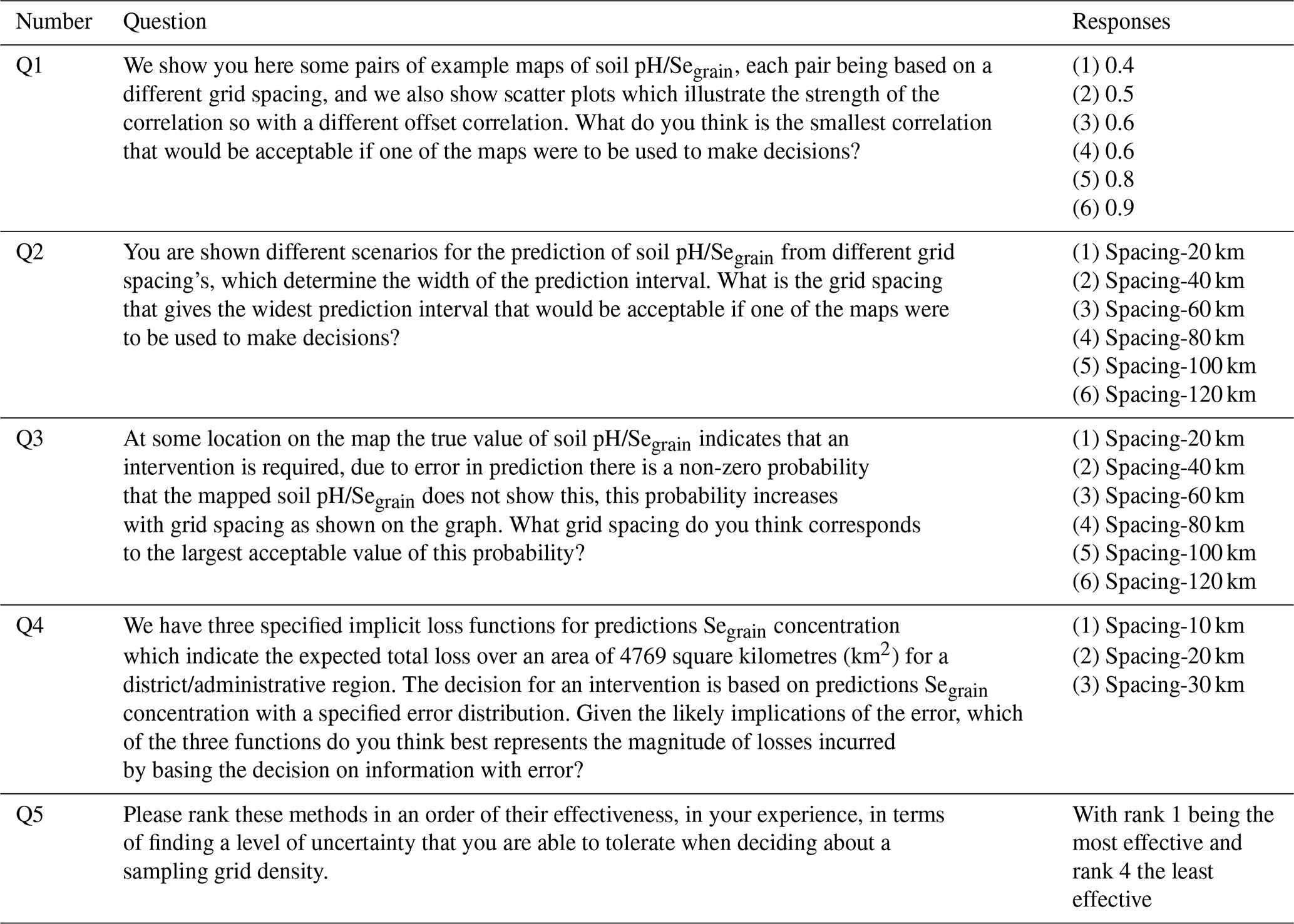
The participants considered each method in turn and were asked to select an appropriate sampling grid density based on the method. Evaluation of the test methods was done through a questionnaire, as shown in Table 1. Using the first four questions, Q1–Q4, we wanted to find out if the method helped the participants to identify a sampling grid spacing. In Q5, we wanted the participants to assess the test methods in terms of their effectiveness regarding the establishment of an appropriate grid spacing. We asked the participants to rank these methods based on their effectiveness with respect to enabling a user to consider the trade-off between sampling effort and the uncertainty in the spatial predictions in the final survey product. We asked them to rank the most effective method as 1 and the least effective method as 4. The participants recorded their responses using an online questionnaire on Microsoft Forms. Offset correlation was the first method presented to the participants. This was followed by prediction intervals and conditional probabilities. The implicit loss function was the final method presented. We started with a measure that we thought all of our stakeholders would most easily understand and then moved on to the more complex methods, so as not to undermine participants' confidence to participate in the exercise.

Table 1 The list of questions used to elicit stakeholder opinions about the set of methods that can help end-users to assess the implications of uncertainty in spatial prediction in as far as this is controlled by sampling.

2.2 Test methods

We used data collected during the GeoNutrition survey; readers are referred to Gashu et al. (2021) and Botoman et al. (2022) for a detailed description of the field sampling. We undertook exploratory analysis of the soil pH and Se_grain concentration using quantile–quantile plots, histograms and summary statistics to check whether there was the need for the transformation of the variables for the assumption of normality. The Se_grain concentration data were skewed, and it was necessary to transform them to natural logarithms. The variance parameters for both the soil pH and Se_grain concentration were estimated by residual maximum likelihood using the likfit procedure in the geoR package (Diggle and Ribeiro, 2010) for the R platform (R Core Team, 2022) with a constant mean as the only fixed effect. These variance parameters were used in the subsequent test methods. The thresholds that we considered in this study for the prediction intervals and conditional probabilities were a soil pH of 5 and an Se_grain concentration of 38 µg kg⁻¹. The threshold for soil pH is 5 in Malawi, such that if the pH at a location falls below 5, it would be necessary to apply lime (Chilimba et al., 2013). The threshold Se_grain concentration is 38 µg kg⁻¹, such that a serving of 330 g of grain flour provides one-third of the daily estimated average Se requirement for an adult woman (Chagumaira et al., 2021). The intervention for soil pH was liming, while the intervention for Se_grain was the provision of fortified food. Selenium is an essential micronutrient with critical roles in human health, and a lack of it can cause thyroid dysfunction and a suppressed immune response (Fairweather-Tait et al., 2011). The methods presented to the participants used the variance parameters modelled above.

2.2.1 Offset correlation

We presented the participants with correlated pairs of hypothetical maps of the soil pH and Se_grain, with differing correlations, so that the extent to which maps might differ as a result of the grid offset could be visualized. We also showed scatter plots that illustrated the strength of the correlation. Figure 1 shows an example of a pair of hypothetical maps of the soil pH and the corresponding scatter plot (see also Figs. S5 and S6). The correlation plots showed the kriging predictions for the soil pH or Se_grain concentration predicted with the variance parameters estimated in Sect. 2.2. We asked the participants to identify the smallest offset correlation that would be acceptable if one of the maps were to be used to make decisions based on the soil or grain property (see Table 1). Neither of the posited pair of maps, based on offset grids, is to be regarded as closer to reality than the other; rather, the question is how consistent they are.

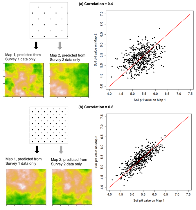
Figure 1 Illustration of the offset correlation (Q1) in two hypothetical cases that use values of 0.4 (a) and 0.8 (b). In each case, the illustrated subset of grid points is of the same dimensions, so the grid is denser in panel (b) than in panel (a). In each case, a hypothetical dataset 1 (black grid points) and dataset 2 (grey points) are collected from grids of shared spacing but offset north–south and east–west by half the grid spacing. The offset correlation is the correlation of the predictions of the soil properties made at common sites from the two grids. In practice, this is calculated theoretically from the variogram and a proposed grid spacing to assess the sensitivity of the original map to variation in the position of the grid origin.

2.2.2 Prediction intervals

Using the variance parameters estimated in Sect. 2.2, we evaluated kriging variances at the centres of cells of square grids of different spacings. We considered minimum and maximum grid spacings of 0.05 and 125 km, respectively, with an increment of 0.5 km. We then computed the cell-centred block kriging variance of the spacings that we were considering by block kriging (Webster and Oliver, 2007). For all of the grid spacings, we computed the cell-centred block kriging variance on 0.01 km² square blocks. We considered three different predictions for each variable, but the prediction interval was fixed, depending only on grid spacing. The three predictions of soil pH were 4.8, 5.5 and 6.0, while predictions of Se_grain were 20, 55 and 90 µg kg⁻¹. These soil pH and Se_grain concentration predictions were presented to the participants using a chart, as shown in Fig. 2.

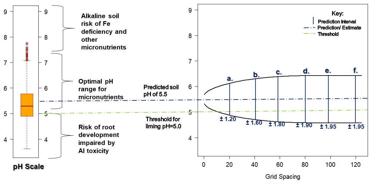
Figure 2 An example of a chart for prediction intervals (Q2) showing the prediction of a soil pH of 5.5 with prediction intervals and in relation to a threshold of pH =5.0.

The chart consisted of (a) a box plot of the distribution of the measured variable based on all soil samples from the study area, (b) a graph of the lower and upper prediction intervals for the prediction at the point of interest for grid spacings from 0 to 120 km, and lines indicating (c) the z_t and (d) the prediction (see Figs. 2, S7 and S8). From the chart, we asked the participants to select the grid spacing that gives the widest prediction interval that would be acceptable if the mapped predictions were to be used to make decisions about soil management or interventions to address human Se deficiency (see Table 1).

2.2.3 Conditional probability

This is a probability that is conditional on the fact that a site requires an intervention (as judged from the true value of the variable being mapped) and that the predicted value at the site does not indicate this. It is a useful measure of uncertainty in a case in which the overall mean value of the variable is such that an intervention would not be recommended; thus, the map is important for identifying locations at which intervention is required. Under these conditions, the probability of this erroneous conclusion increases as the sample grid becomes coarser and the uncertainty attached to the spatial predictions increases. The probability is bounded on an interval [0, 1]. A probability of 1 indicates that the prediction will be equivalent to the overall mean of the dataset. We are not aware that this conditional probability has been used before; thus, its derivation from the geostatistical model is provided in the Supplement.

We presented the participants with a graph of the conditional probabilities plotted against the grid spacing, as shown in Fig. 3 (see also Fig. S9). If the prediction of the Se_grain or pH was below the threshold (z_t), an intervention was needed. We then asked the participant what grid spacing they thought corresponded to the largest acceptable value of this probability (see Table 1).

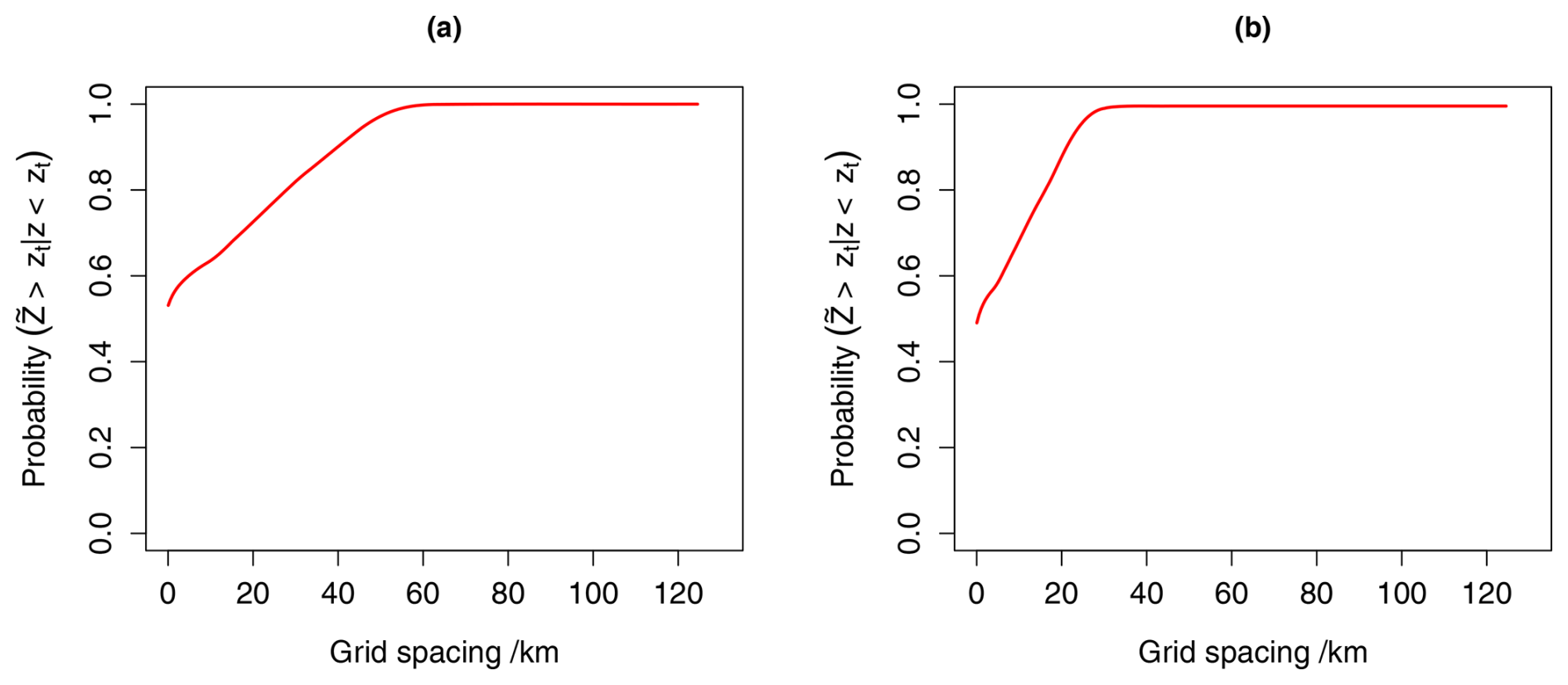
Figure 3 An example of a chart of conditional probabilities (Q3) plotted against grid spacing for (a) soil pH and (b) Se_grain concentration. At a location x₀, $\stackrel{\mathrm{̃}}{Z}$ is the prediction, whereas z is the value of the variable at that location.

2.2.4 Implicit loss functions

In order to compute the implicit loss function, we needed a cost model for the Rumphi District. We used the function defined in Lark and Knights (2015) to return the cost of n samples over an area of A km², i.e. a sample density of $r=N/A$ samples per square kilometre:

$$\begin{array}{}\text{(1)}& C\left(n\right)=\mathit{\omega }+vAr+\mathit{\beta }A{t}_r,\end{array}$$

where ω represents the fixed costs, v is the cost of the laboratory analysis per unit, and β is the field costs per workday per team. The quantity t_r is the time taken to sample per square kilometre at a density of r per square kilometre. We obtained these costs for the Rumphi District by considering the available cost of crop sampling during the GeoNutrition survey conducted in Malawi at a national scale (Gashu et al., 2021; Kumssa et al., 2022). A detailed description of how the cost values were computed is presented in the Supplement.

We fixed the asymmetry ratio at 1.5, assuming that the elicited mean probability threshold from similar stakeholders in Ethiopia and Malawi (Chagumaira et al., 2022) can be regarded as an approximation of P₀, which corresponds to a quantile of the prediction distribution. This implied a bigger loss for an overestimation of the variables (i.e. when the true value of Se_grain is smaller than the prediction, leading to a failure to intervene). With the implicit loss function, we assumed that the sample density is fixed (e.g. on budgetary grounds), and we computed the loss function that would make that a rational choice. We presented three specified implicit loss functions for predictions of the Se_grain for the Rumphi District, with an area of 4769 km² and with sampling densities fixed at 10, 20 and 40 km. Figure 4 (see also Fig. S10) shows the implicit loss function for the Se_grain. We then asked the participants to identify the loss function implied by the sampling decision that looked more plausible with respect to making decisions about interventions to address human Se deficiency (see Table 1).

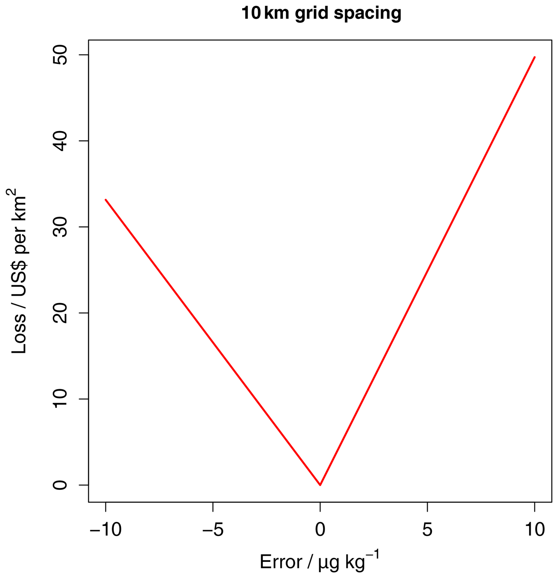
Figure 4 An example of the specified implicit loss functions (Q4) for predictions of the Se_grain concentration at a 10 km grid spacing.

2.3 Data analysis

2.3.1 Test methods

The responses for Q1–Q4 were presented as contingency tables. These tables allowed us to evaluate whether there were differences in the responses of the participants based on (i) the variable used in the test method, (ii) the professional group and (iii) the frequency of use of statistics. We analysed the contingency tables on the basis of a null hypothesis that the distribution of observations between responses (e.g. selected grid spacing) was independent of the factor in the column (e.g. professional group). If evidence was provided to reject the null hypothesis, this would indicate that how a respondent interprets the information presented to select a grid spacing depends on their professional group. A detailed description of how we used the contingency tables to partition the responses of the questionnaire is presented in the Supplement.

The rows of each table correspond to the response (e.g. the different grid spacings), while the columns correspond to the frequency of use of statistics, nested within the professional group and within the variable used (soil pH or Se_grain). Contingency tables allowed us to test the null hypothesis regarding the random association of responses with the different factors in the columns. The expected number of responses under the null hypothesis, e_i,j in a cell [i,j], is the product of the row (n_i) and column (n_j) totals divided by the total number of responses (N). This is the null hypothesis of the contingency table which is equivalent to an additive log-linear model. An alternative to the additive model for the contingency table is the saturated model, which has an extra $(n_{\mathrm{r}}-\mathrm{1})(n_{\mathrm{c}}-\mathrm{1})$ term that allows for interaction amongst the columns and rows of the table. The proportions of observed responses o_i,j may differ from e_i,j in a cell [i,j], and the likelihood ratio statistic or deviance (L) can be used to provide evidence against the null hypothesis. The likelihood ratio statistic is computed as follows:

$$\begin{array}{}\text{(2)}& L=\mathrm{2}\sum _{i=\mathrm{1}}\sum _{j=\mathrm{1}}{o}_{i,j}\log {\displaystyle \frac{o_{i,j}}{e_{i,j}}},\end{array}$$

where L has an approximate χ² distribution under the null hypothesis of random association between the rows and columns of the table, with $(n_{\mathrm{r}}-\mathrm{1})(n_{\mathrm{c}}-\mathrm{1})$ degrees of freedom (Christensen, 1996; Lawal, 2014). We fitted the log-linear models using the loglm function from the MASS package (Venables and Ripley, 2002) for the R platform.

In our study, we wanted to find out if the responses recorded by the participants depended on the variable used (soil pH or Se_grain concentration) or on the background of the respondent. We expected the responses to differ. We thought the participants would have different perceptions of the impacts of the uncertainty for the soil pH and Se_grain concentration. There were more agronomists and soil scientists than public health and nutrition specialists in the meeting, and we expected the priorities of the groups to differ with respect to making decisions on interventions for soil pH and Se_grain concentration. We also thought the frequency of use of statistics would influence the choice of method used to select an appropriate grid spacing.

First, we tested for differences in the responses recorded for each test method, based on the variable used (soil pH or Se_grain concentration), using contingency tables. The responses from stakeholders in different professional groups were pooled within the two variables, as illustrated by pooled Table 1 in Table S5. This gave us a six (number of responses) by two (number of variables) contingency table with 5 degrees of freedom for the questions corresponding to offset correlation, prediction intervals and conditional probabilities (Q1–Q3). However, for the implicit loss function, we did not consider soil pH, as we only had a loss function for the Se_grain concentration.

Second, we considered whether the differences in the responses depended on the professional group of the respondent. Finally, we considered whether the frequency of use of statistics in their job role had an impact on the responses recorded by the respondents. For some questions, we noted a difference in the responses when results were pooled within variable used (soil pH or Se_grain concentration), but there were no differences in responses with respect to the professional group or frequency of use of statistics of the participants for all questions. We further analysed the pooled tables or separate subtables to examine if the responses were uniformly distributed and the null hypothesis was a random distribution. We wanted to test whether the responses of the participants were uniform; i.e. each grid spacing had an equal likelihood of occurrence.

2.3.2 Assessment of the method

The responses for Q5 were tabulated with the methods as the columns and ranks as the rows. The participants ranked their preferred method first. However, to calculate the mean rank (${\stackrel{\mathrm{‾}}{r}}_i$) for each method for all of the respondents, we assigned a score of 4 for the most preferred method and 1 for the least preferred method. We computed the ${\stackrel{\mathrm{‾}}{r}}_i$ for each method for all respondents. We then separated the respondents by their professional group and computed the mean ranks.

Finally, we separated the respondents by their frequency of use of statistics in their job role. Under a null hypothesis of a random ranking for a set of k ranks, the expected mean rank is $(k+\mathrm{1})/\mathrm{2}$. The evidence against this hypothesis is measured by the following statistic:

$$\begin{array}{}\text{(3)}& {\displaystyle \frac{\mathrm{12}n}{k(k+\mathrm{1})}}\sum _{i=\mathrm{1}}^k\left\{{\overline{r}}_i-{\displaystyle \frac{k+\mathrm{1}}{\mathrm{2}}}\right\},\end{array}$$

where n is the total number of rankings and is distributed as χ²(k−1) under the null hypothesis (Marden, 1996).

3 Results

There was a reasonably even spread in terms of the location of our participants (see Fig. S11). About 54 % of the participants constantly used statistics/mathematics within their job role. Only a few participants were educated to the level of certificate/diploma (8 %).

3.1 Test methods

3.1.1 Offset correlation

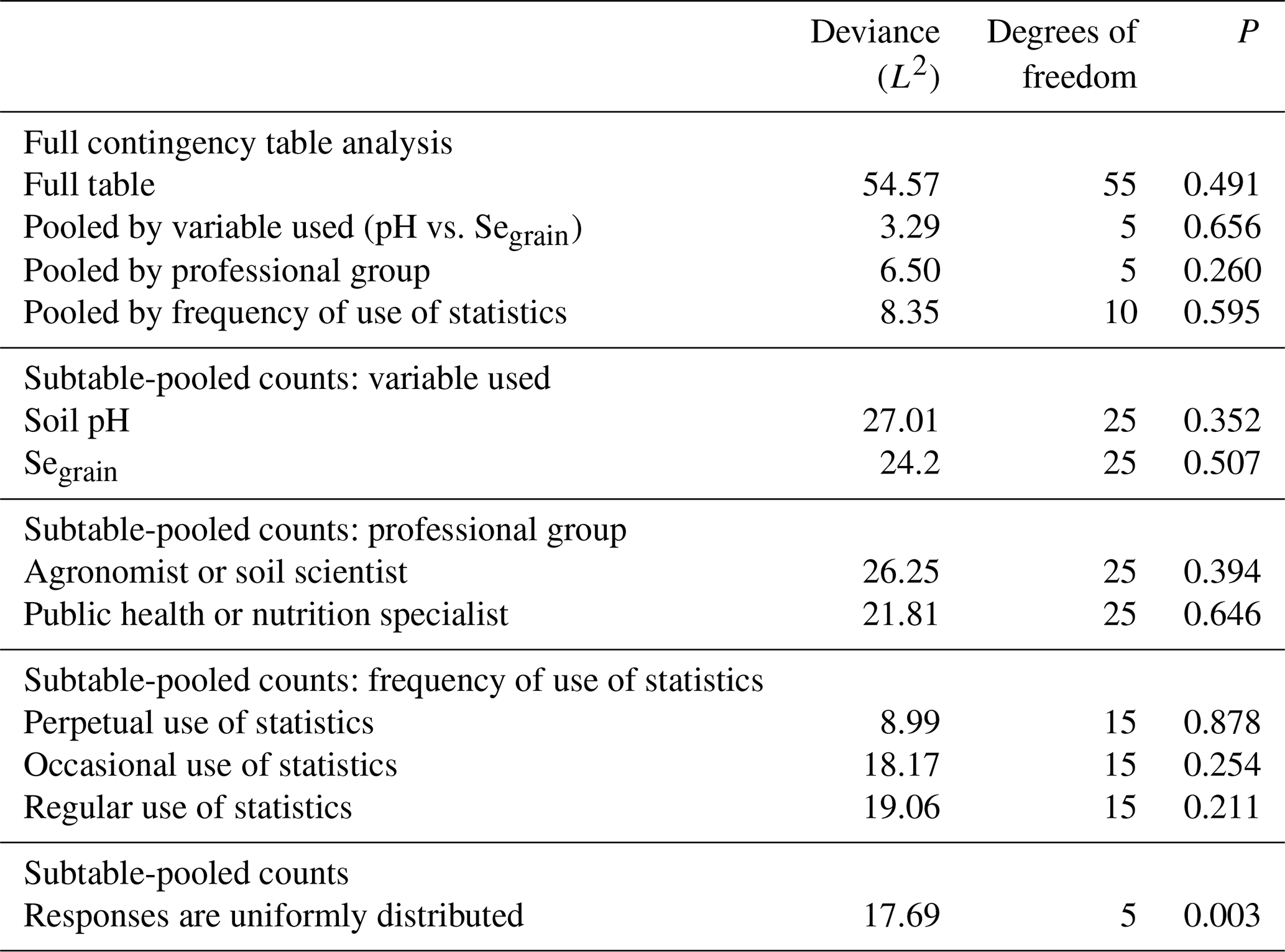
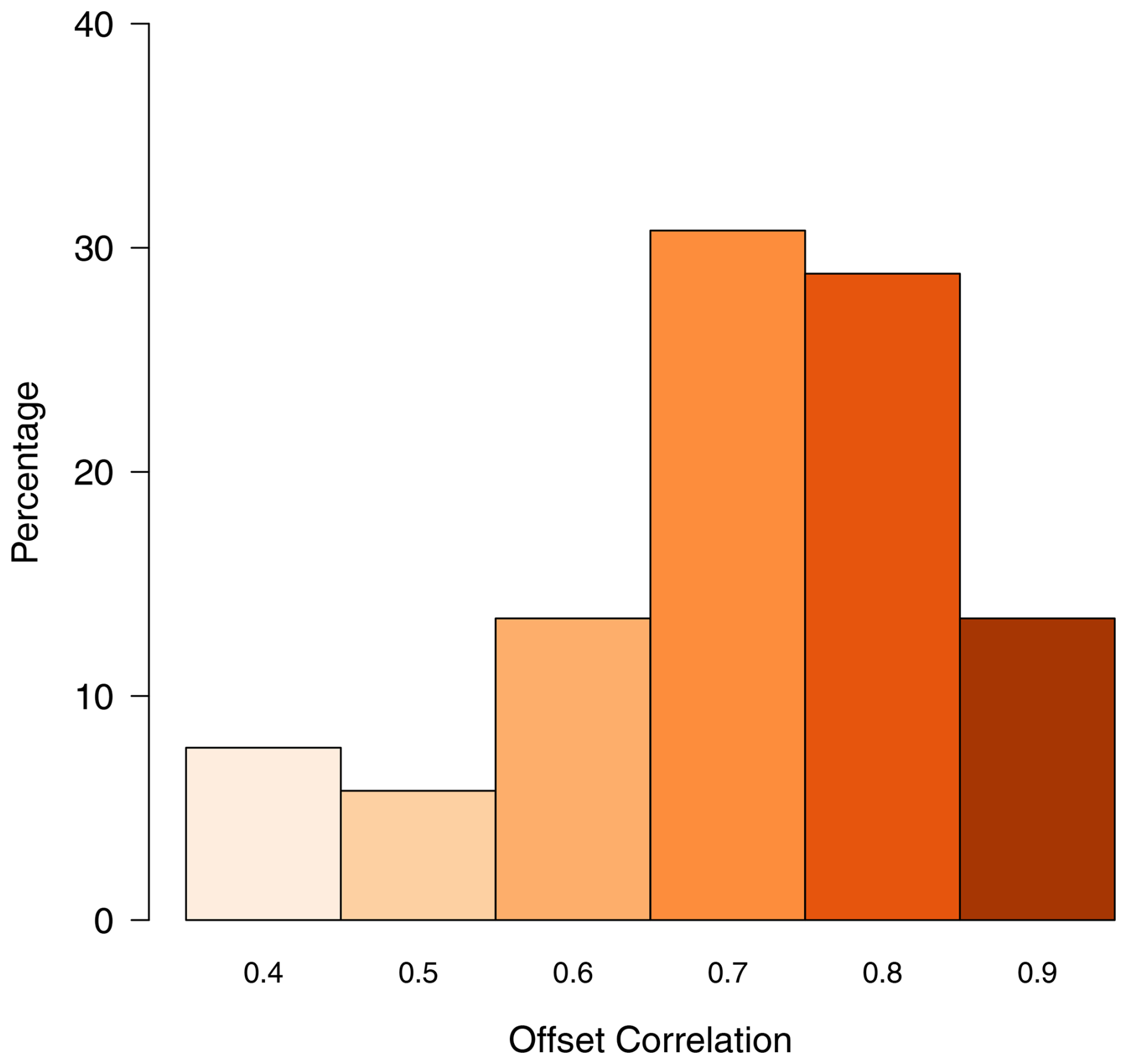
Results for the question on offset correlation (Q1) are shown in Table 2, with the full contingency table given in the Supplement (Table S6). Pooled responses showed strong evidence against a uniform distribution (p=0.003). Figure 5 shows how participants responded to Q1. Most participants selected 0.7 as the minimum acceptable offset correlation if one of the maps was to be used to make decisions based on the soil or grain property. Grid spacings corresponding to this value – 25 km (soil pH) and 12.5 km (Se_grain) – were extracted from plots of the offset correlation vs. the grid spacing (see Fig. S4), based on each variable's variogram.

Table 2 Analysis of the question on offset correlation (Q1) according to the variable used, professional group and frequency of use of statistics.

Figure 5 Bar charts showing how the participants responded to Q1 for offset correlation.

3.1.2 Prediction interval

For further analysis of the question on prediction interval (Q2), we used pooled response counts, as responses did not differ by professional group or frequency of statistical use (Table 3). Figure 6 shows how all participants responded to Q2. For this method, there was no clear preference for grid spacing when sampling soil pH and Se_grain, as there was no evidence against a uniform distribution of responses (p=0.169).

Table 3 Analysis of the question on prediction interval (Q2) according to the variable used, professional group and frequency of use of statistics.

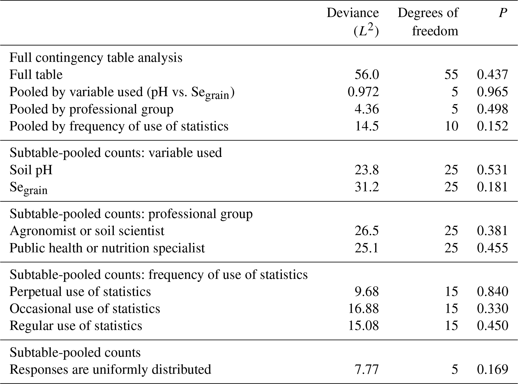
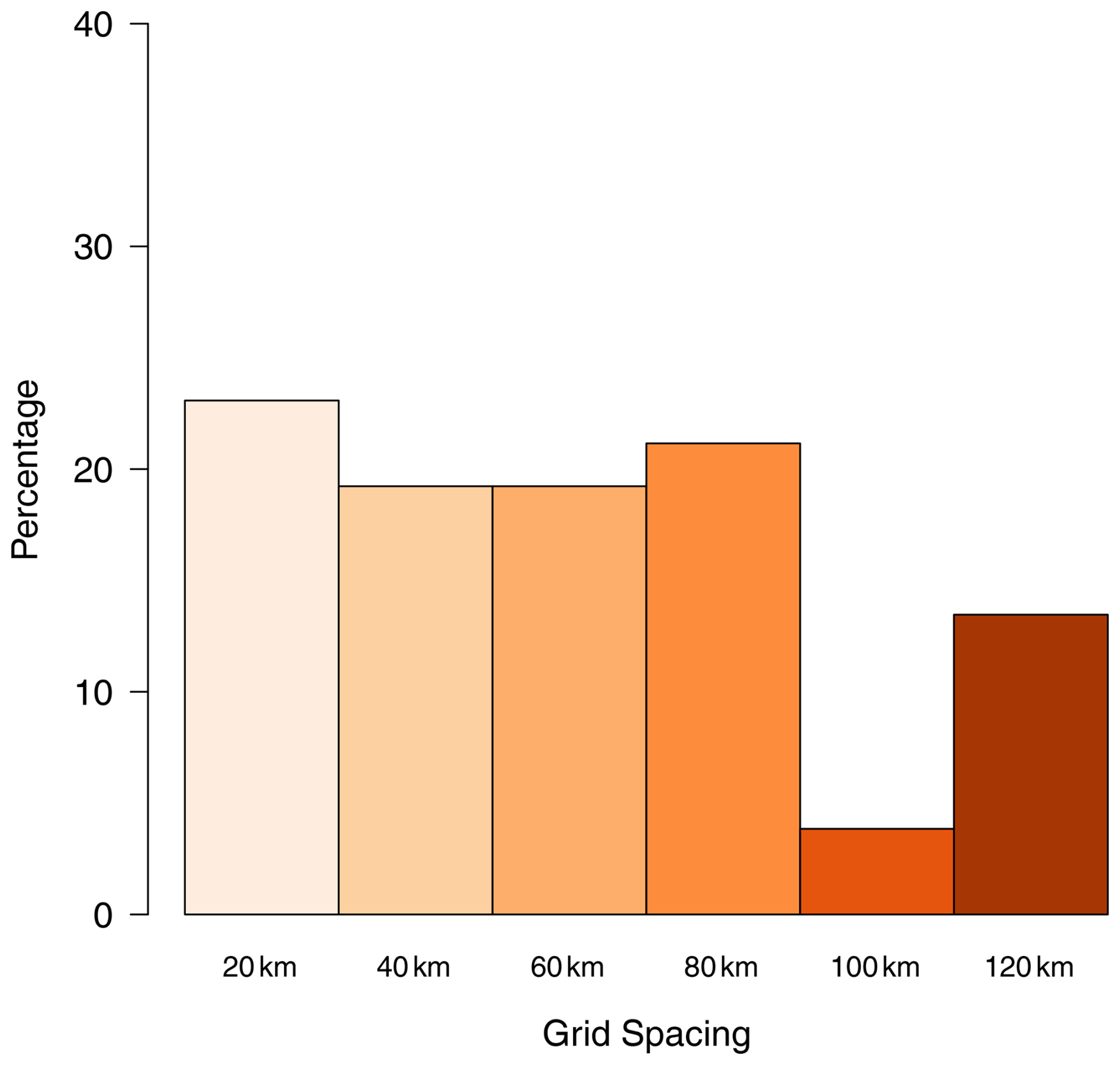
Figure 6 Bar charts showing how the participants responded to the Q2 for prediction intervals.

3.1.3 Conditional probabilities

There were differences in the responses when the columns were pooled by variable (p≤0.001, Table 4), so further analysis was done separately for the soil pH and Se_grain. For both variables, there was strong evidence to reject the null hypothesis that the responses were uniformly distributed (p≤0.001). Figure 7a shows the responses for soil pH (grid spacing: 60 km), whereas Fig. 7b shows the responses for Se_grain (grid spacing: 40 km).

Table 4 Analysis of the question on conditional probabilities (Q3) according to the variable used, professional group and frequency of use of statistics.

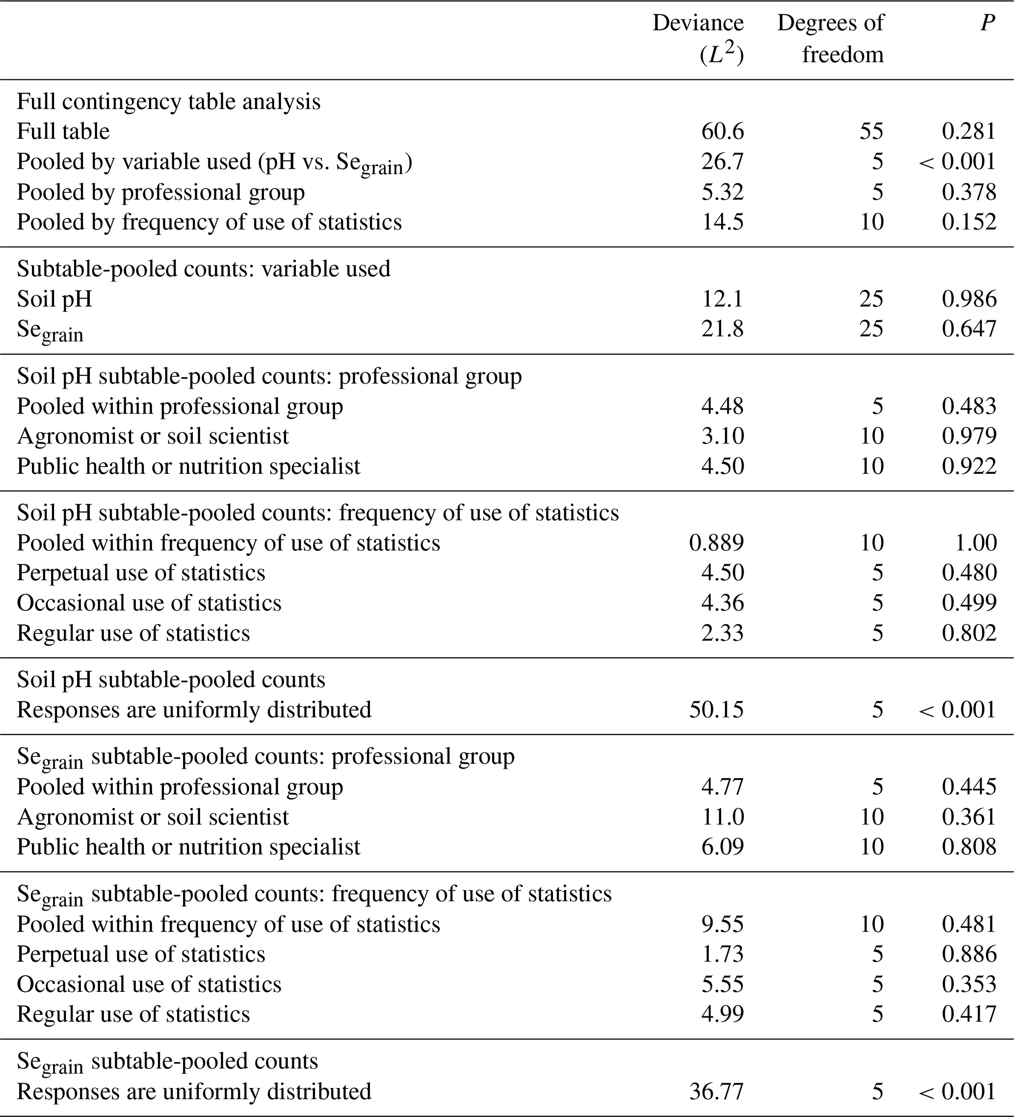
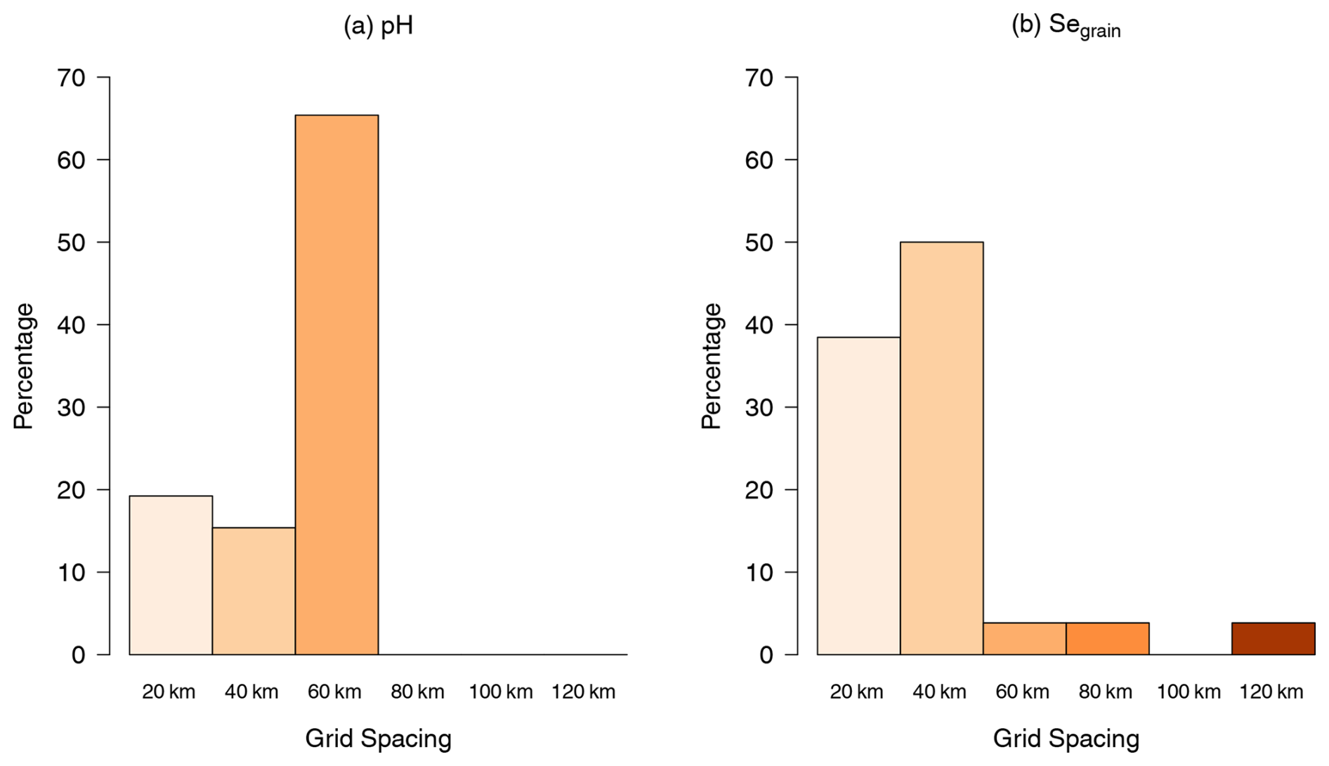
Figure 7 Bar charts showing how all of the participants responded to Q3 on conditional probabilities for the (a) soil pH and (b) Se_grain concentration.

3.1.4 Implicit loss functions

Further analysis of the question on the implicit loss function (Q4) was based on pooled counts of responses (Table 5). There was strong evidence to reject the null hypothesis that the responses were uniformly distributed (p≤0.001). Figure 8 shows the participants' responses to Q4. The grid spacing chosen by the participants for the Se_grain concentration was 20 km.

Table 5 Analysis of the question on the implicit loss function (Q4) according to the variable used, professional group and frequency of use of statistics.

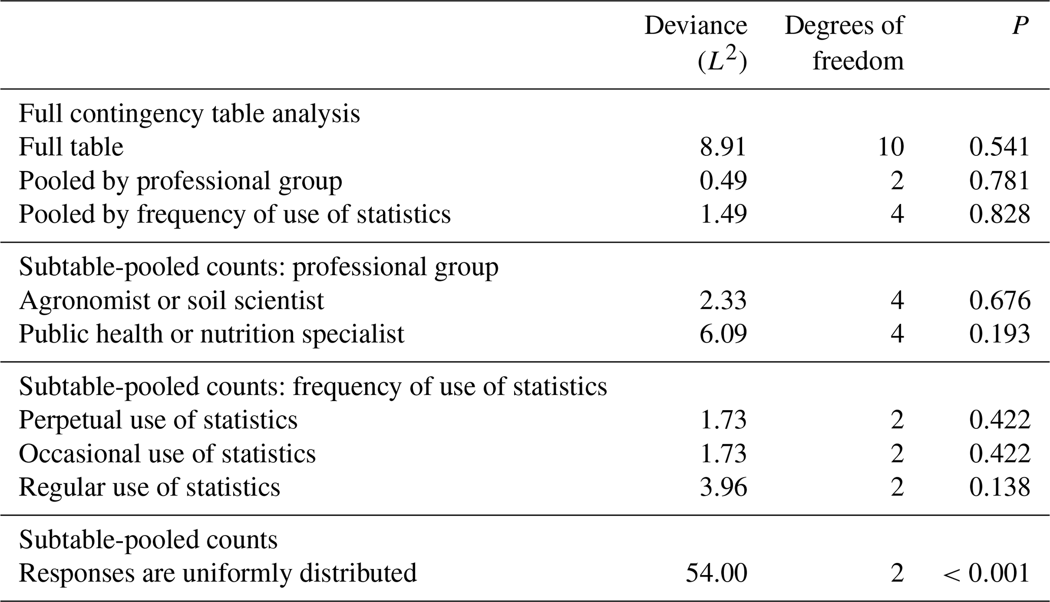
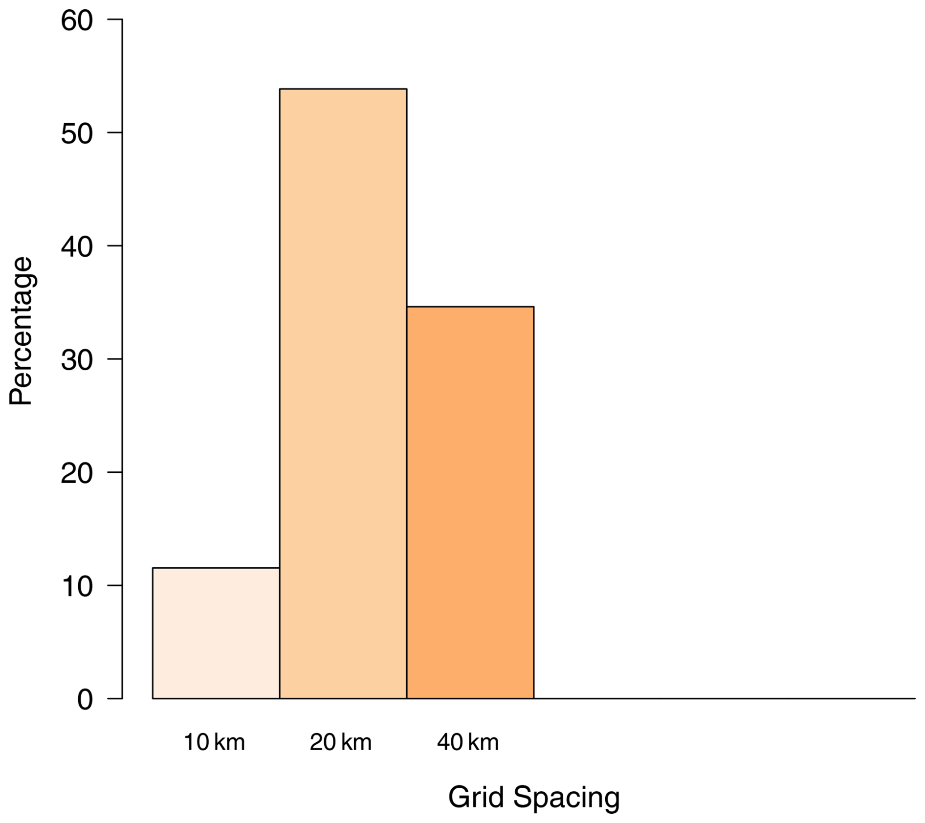
Figure 8 Bar charts showing how all of the participants responded to the Q4 for the implicit loss function.

3.2 Assessment of the test methods

We analysed the responses for Q5 by computing the mean rank values across all participants, by professional group and by frequency of use of statistics; moreover, we tested for evidence against the null hypothesis of random ranking. In all cases, there was strong evidence to reject the null hypothesis of random ranking (p≤0.001; Table 6). Overall, offset correlation was consistently ranked as the most effective method, whereas the implicit loss function was generally ranked as the least effective.

Table 6 Analysis of Q5 according to the professional group and level of use of statistics in the job role.

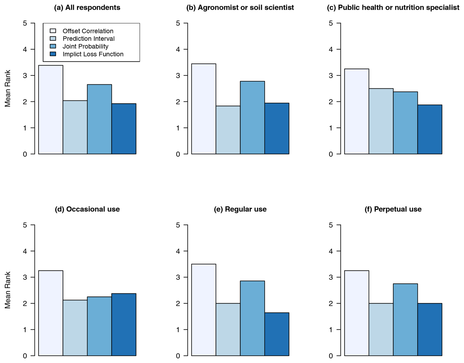
Figure 9 Ranking of test methods in terms of the most effective: (a) by all respondents; by professional group – (b) agronomists or soil scientist and (c) public health or nutritionist specialists; and by frequency of use of statistics – (d) occasional use, (e) regular use or (f) perpetual use.

4 Discussion

In this study, we presented (to groups of information users) four methods (offset correlation, prediction intervals, conditional probabilities and implicit loss functions) that can be used to support decisions on sampling grid spacing for a survey of the soil pH and Se_grain. We wanted to find out if the information users had a preference among the approaches presented to them. Offset correlation was ranked first with respect to the method that stakeholders found easy to interpret (see Fig. 9) in order to make a decision on sampling density. Most respondents (30 %) selected an offset correlation of 0.7, while slightly fewer selected 0.8; thus, over half of respondents are accommodated within this range of values. During the feedback session, information users highlighted that they were more familiar with the concept of correlation, particularly within a closed interval of [0, 1]. This familiarity may have influenced the consistency of the results for this criterion, with over half the respondents selecting 0.7 or 0.8 as a minimum acceptable correlation. This pattern aligns with Hsee (1998), who found that relative measures of uncertain quantities (e.g. size of a food serving relative to its container) are more readily evaluated than absolute measures (the size of serving). Thus, bounded attributes, such as correlation on a [0, 1] scale, can play a more prominent role in an individual's judgement of utility. Hsee (1998) describe this as the “relation-to-reference” attribute. This may explain why offset correlation was highly ranked.

Offset correlation is a more comprehensible criterion for respondents, making it a preferred basis for selecting the sample density in a geostatistical survey over alternatives like kriging variance. Furthermore, it appears to be a measure of uncertainty that participants in the study found comprehensible and were, therefore, able to use to select a grid sample spacing. This measure, offset correlation, recognizes that spatial variation means that maps interpolated from offset grids will differ but that more robust sampling strategies will produce more consistent maps. However, Chagumaira et al. (2021) found that measures of uncertainty related to a specific management threshold of the mapped variable were preferred by participants for the interpretation of uncertain spatial information to general quality measures without a specific management or policy implication. In this case, in contrast, the preferred criterion, the offset correlation, is a general measure of map quality, which is not directly linked to specific interpretation.

Conditional probabilities were ranked second. Using this method, the information users selected spacings where conditional probabilities was 1.0 or very close, i.e. the prediction equivalent to the overall mean. This suggests that the information users may not have fully understood the method. This finding is consistent with the general view that users of information commonly find probabilities difficult to interpret (Spiegelhalter et al., 2011). Because probabilities are bounded [0, 1], the relation-to-reference attribute effect by Hsee (1998) may explain the previous preference for conditional probabilities (Jenkins et al., 2019; Chagumaira et al., 2021), but information users still struggle to interpret them correctly. More work is needed to investigate whether explaining or framing the conditional probabilities in a different way would improve the judgement of their utility by the information users; for example, if the probability was expressed as the probability of an error of omission at a site where intervention is required. More examples and more illustration may be needed in order to “prime” the participants before the exercise. A method might be regarded as easy to interpret because of its form, even when it is not (in this case, a large value of the probability indicated that there was no spatial information in the map to make its predictions better than the overall mean).

Prediction intervals were ranked third by all of the respondents, but there was no evidence against the null hypothesis of random selection among the available spacings. During a feedback session, the information users cited difficulties with respect to assessing the significance of a given prediction interval, given that it can be associated with different prediction values. For very large or small prediction values, the uncertainty is immaterial; it is near the decision threshold that uncertainty becomes important. Similarly, prediction intervals were not highly ranked by information users for communicating uncertainty in maps (Chagumaira et al., 2021). Similar reasons were given by the respondents. We expected that prediction intervals would be of greatest value for the specific interpretation of particular sites but that they would be of limited value for survey planning.

The implicit loss function was the lowest-ranked method. The group of participants also commented that they had difficulties understanding this method, and most people opted for the central value. Loss functions are not readily accessible. It is difficult to define a loss function, as it requires the cost of the errors; moreover, we tried to show information users some consistent approach with some plausible design. The fact that they did not understand the loss functions shows that there is a need for more specific examples to help information users think about loss functions and their implications. It might help the information users if some quantitative information on the following factors was provided: the cost of the survey, the cost associated with intervention campaigns and the cost of the impacts of MNDs on a country's gross domestic product. A reflection of these factors would allow the information user to employ these implicit assumptions when making decisions with respect to selecting a fixed grid spacing to work with (Lark and Knights, 2015).

The background of the information users, i.e. professional group and frequency of use of statistics, had no influence on their responses for all of the methods. However, the background of the information users had an influence on their ranking of the methods in terms of their effectiveness. Offset correlation was ranked as the most effective by all professional groups and by all respondents separated by frequency of use of statistics. Prediction intervals were ranked least effective by those respondents who identified as agronomist or soil scientist but were ranked second by those in public health or nutrition.

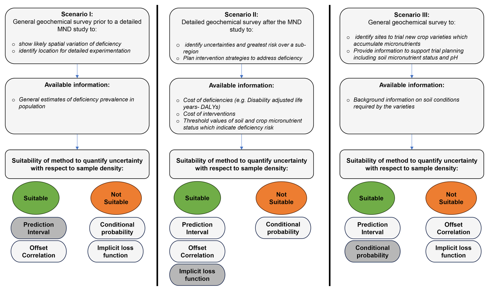
Figure 10 Illustration of the different scenarios of geochemical surveys and the suitability of the methods to quantify uncertainty with respect to sampling densities.

At the beginning of the online workshop, we explained each method with the aid of illustrations. After an explanation of each method, there was a feedback session to allow the participants to seek clarity (from the presenters) on ambiguous and unfamiliar concepts. The participants' questions were answered and explained in different ways by Christopher Chagumaira, R. Murray Lark and Alice E. Milne, with the use of illustrations. However, there are limitations with respect to online workshops. Most participants had their cameras switched off, and the “unconscious” feedback (observing the reactions of participants) usually available to presenters during in-person workshops was unavailable. This unconscious feedback would have prompted the presenter to use a different approach to explain unfamiliar concepts and ambiguous terms. Due to internet connectivity, online workshops were timed, and there was less time for feedback sessions. In such instances, respondents may have sought clarity from the colleagues who had the same interests, resulting in bias (Ball, 2019).

All of the methods may give different results for different variables, as they depend on the variogram of the variable in question. There may be different grid spacings selected for the different variables. A potential problem may exist if the variables were to be sampled in one survey regarding what spacing should be used. This is an important question that needs to be addressed when planning for soil and crop sampling. It may be reasonable to opt for the grid spacing for the variable that is the hardest to characterize. Another option would to consider some minimum quantile over all variables via group elicitation. Black et al. (2008) proposed that a critical subset of soil properties is identified such that the overall sampling scheme is satisfactory for all of the so-called “canary indicators”.

All of the information users recruited in this study were employed in public-sector (e.g. university, civil organization, research and extension) institutes and had experience in their respective fields in a sub-Saharan Africa (SSA) setting. We had no basis for a power analysis to identify a sample size for this activity. Given the exploratory nature of this research, our primary aim was to capture insights from as many relevant participants as possible within each institution. As a result, our major consideration was recruiting individuals willing to participate and with experience at their respective institutions. We therefore attempted to recruit the entire set of suitable respondents in each country. We recognize that the small sample size limits the generalizability of statistical findings. While this study provides insights into participant perspectives by specialism, the lack of demographic information – such as gender, age, location and years of experience – limits the depth of analysis. These characteristics may impact responses; for example, different age groups or experience levels might prioritize certain issues differently. Future studies should consider including these demographic details to explore how such factors influence perspectives, thereby enhancing the robustness of the findings and allowing for subgroup analysis. For this reason, we have interpreted results cautiously and have also incorporated qualitative insights from participants to provide a richer context for understanding these early findings. Moving forward, we plan to include an initial power analysis and possibly extend the study through broader collaborations to enhance robustness.

As we emphasized in our objectives, this study aimed to examine the accessibility of different measures of uncertainty to professional stakeholders. While all of the methods depend on a common linear mixed model for all of the variables, they provide differing, although consistent, information. The different measures would each be most useful for sampling planning for geostatistical prediction to address particular problems. We illustrate this in Fig. 10. Here, Scenario I is a general geochemical survey prior to a detailed MND study and is used to show likely spatial variation in deficiency and to identify a location for detailed experimentation. In this case, there are no specific decisions to be made using the map and no cost (e.g. cost of intervention) linked to the outcomes under consideration. Thus, the implicit loss functions and conditional probabilities (there are no thresholds) will not be useful, whereas the prediction intervals and offset correlation will be very useful. Due to the lack of specificity in the use of the maps and the associated cost, the decision will be relatively straightforward for the range of stakeholders under consideration.

Scenario II is a detailed geochemical survey after the exploratory MND study with the specific objectives of identifying the uncertainties and the greatest risk over a subregion and planning intervention strategies to address deficiencies. Here, prediction errors result in quantifiable losses in accuracy, and the information is essential to guide policy decisions on interventions. Given these considerations, offset correlation will be too general and, therefore, not very useful. The threshold for making intervention decisions is known; therefore, conditional probabilities will be useable and useful. However, there will be a need to (1) invest in specific training for specialists (e.g. public health and nutrition experts) and (2) elicit a probability threshold that represents a consensus model of the losses associated with making a decision with uncertain data. This could follow Chagumaira et al. (2022), who elicited a mean probability threshold for making decisions regarding interventions to address Se deficiency. The implicit loss function will also be useful in this scenario and can be used to judge resource allocation between intervention and general food fortification.

Scenario III is a general geochemical survey to identify sites to trial new crop varieties that accumulate micronutrients and to provide information (such as soil micronutrient status and pH) to support trial planning. Background information on soil conditions required for the varieties is available. In this case, the offset correlation measure is too general to be useful, while implicit loss functions are not relevant. However, conditional probabilities will be very relevant; for example, one could compute the probability that a valuable potential site is not identified. The prediction interval will also be useful in this case, although not as directly as conditional probabilities. There will be a need for training given the challenges that our participants faced with respect to understanding the method, e.g. the use of games and visual examples of everyday problems to build confidence in the interpretation of probabilities to support decision-making.

Note that the events were planned prior to the lifting of all COVID-related restrictions on overseas travel from the UK and on larger gatherings in partner countries. Consequently, participant numbers were limited, and we recognize that these results should not be generalized due to the small sample size. To deepen our understanding, especially regarding the impact of professional grouping, a larger-scale elicitation is recommended. Conducting a face-to-face study would also be valuable to ensure that participants fully grasp the probability concepts – particularly conditional probability – through interactive activities such as games and quizzes before formal evaluation. A practical takeaway is that more time is needed for participants to become familiar with the methods to improve the quality of the elicitation.

5 Conclusions

In this exploratory study, to determine an appropriate sampling density to meet an information user's expectations, we evaluated four methods of communicating the uncertainty associated with kriging predictions made from data from a geostatistical survey. Users of information on soil variation need accessible ways of understanding the implications of the sampling design on spatial prediction and the associated uncertainties. The background of the information user (professional group and frequency of use of statistics) had no influence on the responses selected for each approach. Of the methods that we tested, offset correlation was the most favoured, but it had no direct link to decision-making; moreover, some methods of communication were not well understood (conditional probabilities and implicit loss functions). There were consistent responses with respect to offset correlation – compared to the other methods – and it will likely be more useful to information users with little or no statistical background and to those who are unable to express their requirements with respect to information quality based on other measures of uncertainty. Although previous work has found that the uncertainty in spatial information is best understood when presented in terms of a decision-specific metric, this was not the case here. This shows that more work must be done to develop and elucidate decision-specific approaches, perhaps through methods to elicit useful loss functions. Given the small sample size in this study, there is need for a more in-depth study with a larger sample size to explore these findings further.