the Creative Commons Attribution 4.0 License.
the Creative Commons Attribution 4.0 License.
 | 24 May 2024
Quantifying and communicating uncertain climate change hazards in participatory climate change adaptation processes
Laura Müller
Petra Döll
Participatory processes for identifying local climate change adaptation measures have to be performed worldwide. As these processes require information about context-specific climate change hazards, we show in this study how to quantify climate change hazards with their uncertainties in regions all around the globe and how to best communicate the potential hazards with their uncertainties in order to identify local climate change adaptation strategies. In a participatory process on water-related adaptation in a biosphere reserve in Germany, we used the freely available output of a multi-model ensemble provided by the Inter-Sectoral Impact Model Intercomparison Project (ISIMIP) initiative, which provides global coverage, to quantify the wide range of potential future changes in (ground)water resources. Our approach for quantifying the range of potential climate change hazards can be applied worldwide for local to regional study areas and also for adaptations in agriculture, forestry, fisheries, and biodiversity. We evaluated our approach to communicating uncertain local climate change hazards by means of questionnaires that the stakeholders in the participatory process and the audiences from the general public of two project result presentations answered. To support the stakeholders in participatory climate change adaptation processes, we propose the use of percentile boxes rather than boxplots for visualizing the range of potential future changes. This helps the stakeholders identify the future changes they wish to adapt to, depending on the problem (e.g., resource scarcity vs. resource excess) and their risk aversion. The general public is best informed by simple ensemble averages of potential future changes together with the model agreement on the sign of change. Using or adapting our quantification and communication approach, flexible climate change adaptation strategies can and should be developed worldwide in a participatory and transdisciplinary manner, involving stakeholders and scientists.
- Article
(3563 KB) - Full-text XML
-
Supplement
(480 KB) - BibTeX
- EndNote


Climate change alters environmental systems. Any alteration is likely to be a hazard as humans and other biota have adapted to unaltered conditions, and future alterations are unknown. In combination with the vulnerability of the system under consideration, a climate-change-related physical hazard leads to a risk that should be reduced by adaptation to climate change. As an example, water flows and storages on the continents are changing, and their temporal patterns cannot be assumed to be stationary anymore (Milly et al., 2008). This hazard makes water management, which aims to reduce risks, more difficult as it is based on the evaluation of historic data and is generally adjusted to past conditions (Riedel and Weber, 2020). It is widely accepted that the management of environmental systems worldwide has to be adapted to the changing climate and that robust and flexible climate change risk management strategies should be developed jointly by stakeholders and scientists in a participatory and transdisciplinary manner (Daniels et al., 2020; Döll and Romero-Lankao, 2017; Krueger et al., 2016; Scrieciu et al., 2021; Strasser et al., 2014).
To adapt the current management, stakeholders need to know how the system under consideration may develop in response to climate change. Given that adaptation to climate change impacts always pertains to the future, uncertainty is unavoidable (Lux and Burkhart, 2023). While some effects of climate change, such as an increase in temperature or an increase in precipitation variability, are qualitatively well known, the quantification of changes, in particular for areas with a small spatial extent, is highly uncertain due to the complexity of the Earth system, as well as the unpredictability of future greenhouse gas emissions (Döll et al., 2015). Uncertainty means that we have limited knowledge about something (Marchau et al., 2019); i.e., “[it] is the inability to determine the true magnitude or form of variables or characteristics of a system” (Mahmoud et al., 2009, p. 806). This is why (a) future changes should be assessed with their uncertainty, and (b) a suitable visualization should be found with which the future changes, along with their uncertainty, can be communicated.
Future changes are quantified with climate and impact models (Appendix A2) but only with a rather large degree of uncertainty (Lange et al., 2020). Assuming the same greenhouse gas emission scenarios, different climate models compute rather different future changes in climatic variables such as near-surface temperature and, in particular, precipitation, and different impact models will translate the same time series of climatic input variables into rather different time series of, e.g., discharge (Tabari et al., 2021). It is the state of the art to estimate the uncertainty of future changes by analyzing the output of multi-model ensembles (Döll et al., 2015). Multi-model ensemble output is the output of multiple impact models, where each of the impact models is run various times driven by the output of multiple climate models. The output of each climate model–impact model combination can be considered to be equally likely as it is, in most cases, impossible to say which of the models, each with different model algorithms and input data, provides a better representation of reality compared to the other models. Thus, for each future change, the distribution of the changes simulated by all model combinations can be used to quantify the uncertainty of future changes caused by the uncertainties of climate and impact models, and these uncertainties can be classified as “shallow” (Döll et al., 2015; Döll and Romero-Lankao, 2017). In contrast, pathways of future greenhouse gas emissions are characterized by “deep” uncertainties such that their occurrence cannot be described by probabilities, and it is not even possible to rank them by their likelihood (Döll and Romero-Lankao, 2017). This level of uncertainty can be addressed by generating scenarios of alternative plausible futures. Therefore, for most evaluations, it is preferable to analyze separate multi-model ensembles for each emissions scenario. To confront various origins of uncertainties when modeling the future, Maier et al. (2016) suggested that the quantification of potential future changes should be based on the combination of three complementary paradigms, which are “(a) anticipating the future based on best available knowledge, (b) quantifying future uncertainty, [and] (c) exploring multiple plausible futures” (Maier et al., 2016, p. 155, Fig. 1). Thus, it is essential to characterize the uncertainty of simulated changes that is caused by the multiple plausible future greenhouse gas emissions and the uncertainties of the applied climate and impact models (Riedel and Weber, 2020).
The Inter-Sectoral Impact Model Intercomparison Project (ISIMIP, http://www.isimip.org, last access: 15 May 2024) provides freely available multi-model ensembles of many model output variables that are of interest in quantifying climate change hazards in several impact sectors (water, lakes, biomes, forests, permafrost, agriculture (crop modeling), energy, health, coastal systems, fisheries and marine ecosystems, and terrestrial biodiversity; ISIMIP, 2019). The available impact model outputs mostly cover all land areas of the globe. For each impact variable, ISIMIP2b provides a time series for historic and future periods and several greenhouse gas emission scenarios, which were computed by multiple global impact models (Frieler et al., 2017), with which the uncertainties of future changes in impacted variables can be characterized.
To support stakeholders who are responsible for identifying and performing robust and flexible local climate change risk management, experts need to translate the multi-model ensemble output into meaningful and usable information (Daniels et al., 2020). A communication framework for epistemic uncertainty has been developed that “addresses who communicates what, in what form, to whom, and to what effect while acknowledging the relevant context as part of the characteristics of the audience” (van der Bles et al., 2019, p. 3). Of the three formats to communicate uncertainty, numerical and visual formats convey a higher precision of uncertainty, while a low-precision uncertainty is typically communicated verbally. Limited empirical evidence exists on which communication formats are more suitable – the available evidence mostly concerns how verbal expressions are interpreted, but there is very little on visual and numerical formats (van der Bles et al., 2019). While a wide variety of approaches – in particular, visualization approaches – have been developed to communicate uncertainty, the most suitable format of uncertainty communication depends on the communicators' objectives, communication context, and audience, and no general recommendations for the perfect communication format in a certain context can be given (Spiegelhalter et al., 2011).
To communicate the quantified potential changes with their uncertainties visually, a suitable visualization format is needed and should not be translated into median or mean changes only as this would suppress information about the actual uncertainty range of projected changes. Suitable ways to communicate and assess the potential range of future developments and thus identify the consequent adaptation needs should be identified, e.g., by analyzing risks under a discrete number of likely future developments of the physical system (Jack et al., 2020). Crosbie et al. (2013) suggested showing the distribution of future changes in groundwater recharge to stakeholders in Australia so that, depending on their risk aversion, they can decide which future changes they want to adapt to. Representation of spatially heterogeneous changes and their uncertainties is often done by showing maps with the mean of a multi-model ensemble, as well as what fraction of the models agree on the sign of change (decrease or increase); such a representation of uncertainty is not very helpful for climate change adaptation as a high agreement on the sign of change may be due to a range of model projections of, e.g., −20 % to −30 % or −5 % to −50 %. Model-based uncertainty of future changes in a variable for a certain spatial unit is often visualized by boxplots (Tukey, 1977) that show the percentages of all ensemble members that exceed a certain change in the variable (e.g., Arias et al., 2021). Boxplots are challenging to comprehend due to the difficult interpretation and the non-unique definition of the “whiskers”, with one definition being that the whisker length corresponds to 1.5 times the interquartile range; in addition, the handling of outliers is not fixed. To provide information about the range of possible future changes in meteorological changes in Germany, the Climate Service Center Germany (GERICS) uses bar charts with the whole range of changes projected by the different ensemble members, showing, in addition, the median and the 20th (P20) and 80th (P80) percentiles, e.g., in their Climate-Fact-Sheets for Regions (available under https://www.climate-service-center.de/, last access: 15 May 2024). Similarly, the letter-value plot (Hofmann et al., 2017) shows several percentiles with bars, but the more reduced the bar width, the more distant the percentile is from the median. To show the distribution of values, violin plots (Hintze and Nelson, 1998) can be used, which also show the minimum, median, and maximum values. Considering the numerous uncertainty visualization formats, a suitable format has to be identified for climate change adaptation processes.
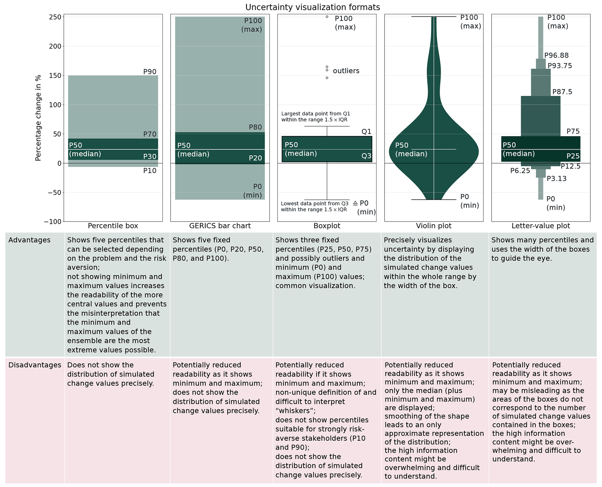
Figure 1The uncertainty visualization formats of percentile box, GERICS bar chart, boxplot, violin plot, and letter-value plot, as well as their advantages and disadvantages, used to communicate uncertain changes to stakeholders. All represent the distribution of changes that are simulated by the different members of the multi-model ensemble and indicate the change values that are not exceeded by a certain percentage (percentile) of the ensemble members. These uncertainty visualization formats exemplarily show the potential percentage changes in groundwater recharge in the BRR in the winter months in the far future around 2084 under the emissions scenario Representative Concentration Pathway (RCP) 8.5 as simulated by 28 multi-model ensemble members. The script and an example data set for this comparative figure of uncertainty visualization formats for the same data are freely available (Müller, 2023). Q1: first quartile (≜ P25); Q3: third quartile (≜ P75); IQR: interquartile range, i.e., range between Q1 and Q3.
Clear and precise communication on the uncertainty of future climate change is required to avoid biases and misunderstandings, and experts need to clarify the causes of the uncertainty and how uncertainty was determined (van der Bles et al., 2019; Kloprogge et al., 2007). Experts should consider the so-called “usability gap”, the gap between the information that knowledge producers (i.e., experts) perceive to be useful and the information that knowledge users (i.e., stakeholders) consider to be usable in their daily work (Lemos et al., 2012). Only if knowledge users consider the information of, e.g., future hazards and their inherent uncertainty to be usable will they include it in their decision-making process. “[U]sability depends on three interconnected factors: users' perception of information fit, how new knowledge interplays with other kinds of knowledge that are currently used by users, and the level and quality of interaction between producers and users” (Lemos et al., 2012, p. 789). In general, multiple formats should be used to address a diverse audience, including words and numbers in graphs, along with narratives, images, and metaphors; when communicating with the general public, it is important to assume low numeracy (Spiegelhalter et al., 2011). As the characteristics of the audience, such as a priori beliefs and values, affect how uncertainty communication is received, communication should be adapted to it (Corner et al., 2018; van der Bless et al., 2019). Emphasizing uncertainty alone may discourage and create hesitancy among the audience, making it crucial to also explain areas of high scientific consensus (Corner et al., 2018). Scientists might be afraid that communicating uncertainty reduces trust, but the communication of “(epistemic) uncertainty does not always have a negative effect on people's affective states” (van der Bles et al., 2019, p. 27). Finally, if experts communicate uncertainty issues well, stakeholders might gain an enhanced understanding and acceptance of model results, as well as of adaptation measures (Parviainen et al., 2020).
The objective of this study is to show how to quantify climate change hazards with their uncertainties for any region around the globe from publicly available ISIMIP multi-model outputs and how this information can be communicated in a participatory process as a starting point for identifying local climate change adaptation strategies. While the communication approach was evaluated, no concrete conclusions can be drawn due to the small number of evaluating participants in a participatory process (26 evaluating participants). We utilize experiences from transdisciplinary research on freshwater-related adaptation to climate change in a biosphere reserve. The research project KlimaRhön aimed to develop, in a participatory process with local stakeholders, climate change adaptation strategies that enable society and freshwater ecosystems to sustainably use the changing water resources in the UNESCO biosphere reserve Rhön (BRR) in Germany. In the project, we quantified and communicated future changes in total runoff and groundwater recharge and their shallow and deep uncertainties as derived from a freely globally available multi-model ensemble of global climate models (GCMs) driving global hydrological models (GHMs) at the very beginning of the participatory process.
Methods to visualize the uncertain impacts of climate change are presented in Sect. 2. The approaches for quantifying and communicating the uncertainty of climate change-induced hydrological hazards are described in Sect. 3. In Sect. 4, we present the evaluation of our communication formats. We discuss our results in Sect. 5 and finally draw conclusions in Sect. 6.
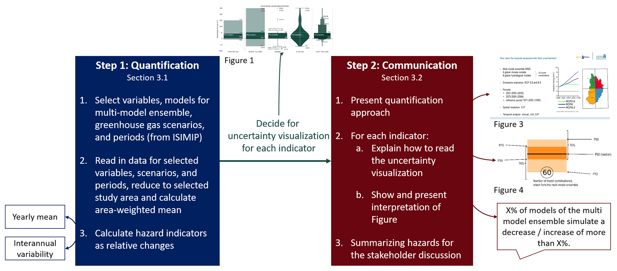
Figure 2Schematic of the presented approach of quantifying and communicating uncertain climate change hazards in participatory climate change adaptation processes. ISIMIP: The Inter-Sectoral Impact Model Intercomparison Project (https://www.isimip.org/, last access: 15 May 2024). In the figure with the caption “Figure 3”, the left figure was modified from a figure in van Vuuren et al. (2011, pp. 23–24), and the left logo in the top-right part was created by Max Czymai.
Depending on the communication objective and the degree of intended precision, uncertainty can be communicated and visualized, among other things, with the bar charts used by GERICS, boxplots, violin plots, or letter-value plots (Fig. 1). For a low degree of required uncertainty precision, only the range of uncertainty with the minimum and maximum values could be communicated. Higher precision can be achieved by subdividing the total range into percentiles (GERICS bar charts, boxplots) that show the change values that are not exceeded by a certain percentage of the ensemble members. Uncertainty is visualized most precisely by violin plots, which display the distribution of values within the whole range by the width of the box; smoothing of the shape, however, leads to an only approximate representation of the distribution. The higher the communicated uncertainty precision, the more information is transported, which again might be overwhelming for the end user.
We came up with our approach of graphics resembling those of GERICS, which we refer to as percentile boxes, because we did not want to communicate minimum and maximum values (1) to not give too much room to possible outliers and (2) to not give the impression that minimum and maximum values could not be exceeded in reality. We wanted to have several percentiles to transparently visualize uncertainty to stakeholders and to enable communication of more thresholds than other visualization formats. In this way, the communicator has the opportunity to say what percentage of models simulated a stronger or weaker change than a certain change value, which supports communication that does not include a specific prediction. Another advantage is that the percentiles can be chosen individually depending on the risk aversion and the problem (Fig. 1). Stakeholders would like to know about (almost) worst-case future changes but maybe not the most extreme results and thus not the outliers of the ensemble. For our percentile boxes, we arbitrarily defined the upper and lower 10 % of the multi-model results as outliers and therefore did not display them.
Figure 1 shows the advantages and disadvantages of visualization formats (including the percentile box) that we identified for the communication of uncertainty to stakeholders. To improve the letter-value plot to communicate uncertainty in participatory processes, fewer and specifically selected percentiles should be shown; however, the distribution of values is still misleading (Fig. 1). When displaying minimum to maximum values, and if the focus of the communication is on the distribution of values, we would recommend using violin plots to prevent outlier values from being misinterpreted as being as frequently simulated as values within the P10 to P90 range. As the violin plot only indicates three percentiles (the median, minimum, and maximum values) with a line, it may more easily induce the viewer to interpret the median as the best estimate and disregard the uncertainty in the consequent adaptation decisions. Therefore, violin plots are less suitable for participatory processes than percentile boxes. However, suitability can be improved when the violin plot is supplemented with more percentiles with lines. The percentile box, GERICS bar chart, boxplot, and letter-value plot could be supplemented with points displaying the change values to show the distribution of values.
Future changes should be quantified with their uncertainty, and then a suitable visualization should be found with which the future changes, along with their uncertainty, can be communicated in participatory climate change adaptation processes; this is an approach that we applied (Fig. 2). At first, scientists or experts have to decide on what climate change hazard information to produce and how to produce it (Fig. 2, Step 1), along with how to visualize the information (Fig. 2, arrow between the boxes), before they communicate it to local stakeholders (Fig. 2, Step 2). Thus, during the first step, the quantification, they need to decide what indicators of climate change hazard should be quantified given the problem, the interest of the stakeholders, data availability and quality, and technical and time constraints. In the second step, the scientists, experts, or communicators have to decide on what to communicate, with which visualization format to communicate, and how to communicate given their audience, the aim, and the generally severe time constraints in the participatory process. Thus, this approach partially follows the framework for uncertainty communication of “who communicates what, in what form, to whom, and to what effect” (van der Bles et al., 2019, p. 3). In our study, we did not consider the option of not communicating our analyzed results ourselves. In Sect. 3.1, we explain “what is communicated” (Fig. 2, Step 1), and in Sect. 3.2, we elaborate on “in what form [it] is communicated” (Fig. 2, Step 2). It was evident “to whom” we communicated, i.e., that our communication targeted local stakeholders from our study area (Sect. 3.2.1), who have diverse (experiential, educational, and professional) backgrounds. Our objective (“to what effect is [it] communicated”) was to raise awareness about uncertainties, enabling stakeholders to make more informed decisions in their respective roles and to engage in better discussions during the subsequent workshops in the participatory process of the project KlimaRhön.
The terms and concepts used in the field of climate change risks and adaptation have different definitions in different contexts. To ensure mutual understanding and alignment, we recommend clarifying the definition of central ambiguous terms with stakeholders according to Table A1 in the Appendix.
3.1 Quantification of hydrological hazard indicators
Changes in the hydrological variables of total runoff and groundwater recharge were used to inform local stakeholders about potential future hydrological changes in the study area. The long-term average total runoff of a region corresponds to the renewable water resources in this region (Döll et al., 2015). It is comprised of two components, namely groundwater recharge and surface runoff (Ertl et al., 2019). Groundwater recharge is the component of total runoff that replenishes the groundwater, and its long-term average is the renewable groundwater resources (Ertl et al., 2019). Groundwater was analyzed in addition to total runoff as water supply in the BRR mainly depends on groundwater.
To assess the potential impact of future climate change on total runoff and groundwater recharge in the BRR, we used the output of a GCM–GHM multi-model ensemble that consists of eight GHMs, each of which was driven by the bias-adjusted output of four GCMs, which resulted in an ensemble of 32 model combinations, i.e., ensemble members (for more details, see Appendix A3). These multi-model outputs are provided by ISIMIP (ISIMIP 2b, https://www.isimip.org, last access: 16 May 2024; for more details, see Appendix A4) and have a spatial resolution of 0.5° latitude by 0.5° longitude (55 km × 55 km at the Equator) and varying temporal resolutions depending on the impact variable (ISIMIP, 2019). We used the output of the GCM–GHM multi-model ensemble for two reasons: (1) there exists no regional hydrological model that could be applied for climate change assessments, and (2) the application of a single regional model might not decrease the uncertainty but could lead to an underestimation of uncertainty as the uncertainty of hydrological models regarding the translation of climate change into hydrological change would be neglected (Davie et al., 2013; Reinecke et al., 2021). We processed, analyzed, and communicated the output variables of groundwater recharge (monthly resolution; the variable name “qr”) and total runoff (daily resolution; the variable name “qtot”), with the latter being to compute total water resources.
In the first step, we processed the data by reading in the NetCDF files for the hydrological variables of total runoff and groundwater recharge, structuring the needed data, and saving them in an extra file. From the original ISIMIP NetCDF file, we selected the data only of the four grid cells overlying the BRR (Fig. S1 in the Supplement) and of two chosen greenhouse gas emissions scenarios, as well as for the reference period 1971–2000 and two future 30-year periods – the “near future around 2035” (2021–2050) and the “far future around 2084” (2070–2099), which were chosen with our project partners, the administrative offices of the BRR, to ensure comparability with their studies and a German climate projection ensemble project (Hübener et al., 2017; Appendix A5). Emissions scenarios represent the substantive epistemic uncertainty of future human activities affecting greenhouse gas emissions (Döll and Romero-Lankao, 2017; Table A1). We used the two Representative Concentration Pathways (RCPs) 2.6 and 8.5 (for more details, see Appendix A6) to inform stakeholders about two possible courses of anthropogenic emissions.
In the next step, the monthly or daily data were aggregated into yearly averages of annual and seasonal flows. As for seasons, we decided on the summer months (June, July, August) and the winter months (December, January, February) because (1) in the BRR climate change tends to decrease summer runoff and increase winter runoff (Schönthaler and Andrian-Werbung, 2008), and (2) there is a high public awareness of drying summers due to the recent summer droughts (Sect. S1 in the Supplement). To not overwhelm the audience, i.e., the stakeholders, with too much information, we decided not to analyze the spring and autumn months.
With these annual and seasonal yearly means, we first calculated area-weighted averages (Appendix A7), and then we either calculated a mean over each period or sorted the values of each period according to magnitude for the analysis of interannual variability. The 30-year mean was calculated to give the stakeholders an overview of the future change tendencies. The 30-year mean values were calculated for the two future periods and the reference period with both the annual averages and the seasonal averages of the summer and winter months. Climate change might lead to a higher interannual variability, which would mean that, e.g., the relative decrease in water resources during a dry year may be higher than the average decrease. To additionally show this to the stakeholders and to make them aware of how the interannual variability of total runoff and groundwater recharge may change due to climate change, all 30 yearly values of each 30-year period (the two future periods and the reference period) were sorted according to their magnitude, resulting in exceedance probabilities (for more details, see Appendix A8).
In the next step, the future-period mean values and the sorted values of each future period were converted to percentage changes with the historical values (Appendix A9) because the analysis of relative changes is more robust than the analysis of absolute values, one reason for this being the low accuracy of GCMs and GHMs when simulating current climate conditions. In the last step, the values were partitioned into three different multi-model ensembles of projected changes. For the far future, the RCP 2.6 multi-model ensemble with 32 model combinations and the RCP 8.5 multi-model ensemble with 28 model combinations are used; one GHM did not provide simulations for RCP 8.5 (Appendix A3). For the near future around 2035, we analyzed the results of RCP 2.6 and RCP 8.5 together as one multi-model ensemble of the total 60 ensemble runs. This is appropriate because climate change until 2035 does not depend much on the emissions scenario, and by combining the outputs, the changes and their uncertainties are more robust.
3.2 Communication of climate change hazards
The goal is to communicate the computed hazard indicators, i.e., the potential future hydrological changes, in a way that they become usable information for stakeholders. This requires a good understanding of the uncertainties of the model results and the relevance of these uncertainties to climate change adaptation. Due to the diverse academic backgrounds of stakeholders in participatory processes, our objective was to effectively communicate the quantification and the potential hydrological hazard indicators in a way that would also be accessible to stakeholders with limited educational backgrounds.
We presented the quantification method and computed hazard indicators related to groundwater recharge and total runoff during a 30 min plenary session with 31 stakeholders in the participatory process (Sect. 3.2.1). To compare this communication format, we presented the same hazard indicators and their analysis to two audiences interested in the results of the project KlimaRhön in 2023 (Sect. 3.2.1) in two alternative ways, namely the proposed way applied in the participatory process (see “Communication of potential changes in 30-year mean values by percentile boxes” to “Summarizing hazards for the stakeholder discussion”) and a more common way following the IPCC (Arias et al., 2021; see “Alternative communication of potential changes of 30-year mean values by tables”).
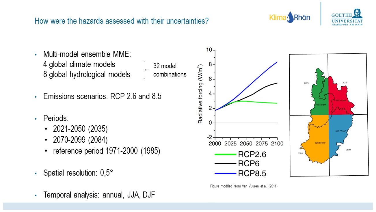
Figure 3With this slide (the original slide was in German), the quantification of the hydrological hazard indicators (Sect. 3.1) was explained to the stakeholders in the first workshop. RCP: Representative Concentration Pathway; JJA: June, July, August; DJF: December, January, February. The left figure in the slide was modified from a figure in van Vuuren et al. (2011, pp. 23–24), and the left logo in the top-right part was created by Max Czymai.
3.2.1 Participatory process
The aim of the transdisciplinary project KlimaRhön was to develop freshwater-related strategies for adaptation to climate change considering the well-being of both humans and the biota in springs and streams. An interdisciplinary team of two sociologists and us, two hydrologists, designed and conducted the participatory process. The stakeholders represent a wide range of sectors including agriculture, nature conservation, political decision-makers (mayors), administration, industry, water supply entities, and non-governmental organizations. The key stakeholders are the three administrative offices of the BRR, one for each federal state.
The participatory process comprised several interviews, five workshops, and three focus groups. The first, second, and third workshops took place in February, May, and October 2021 in the form of video conferences, while the fourth and fifth workshops took place in June and November 2022 in the BRR. Before the first workshop, interviews with 22 stakeholders were conducted, where their problem perspectives on climate change risks regarding freshwater were elicited. The aim of all the workshops was that stakeholders jointly develop climate change adaptation strategies, learn about other perspectives, and network.
The quantification of the potential hydrological changes and its communication method were set up disciplinarily by us, the hydrologists in the team, before the participatory process. The potential hydrological changes were only communicated in the first workshop in the participatory process, which had the character of a kick-off meeting. A total of 31 stakeholders participated to learn about potential future changes in renewable groundwater resources and total renewable water resources through a presentation and to identify a problem in the form of one or two specific adaptation field(s) in a World Café. The stakeholders, except two, were not accustomed to working with climate change information, and they were not familiar with assessing uncertainties using multi-model ensembles.
After the participatory process of the project KlimaRhön had finished, we presented its results (including the quantified potential changes in water resources, workshop methods, and participatorily identified adaptation measures) in June 2023 to an expert group of seven managers of inter-municipal alliances and municipal climate change managers (in the following referred to as the in-person presentation). In July 2023, 67 persons attended an online presentation, in which we again presented the project results; this presentation was open to everyone, was free of charge, and included mainly citizens but also actors from administration, as well as members of the administrative units of the BRR.
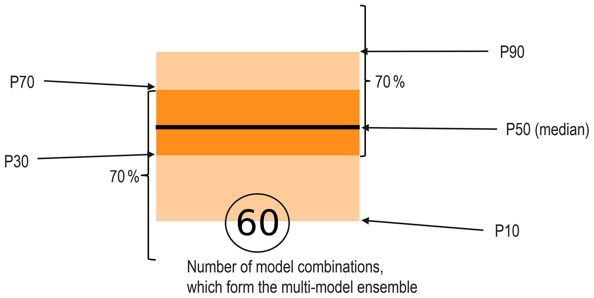
Figure 4Schematic for the explanation of the percentile box, the first diagram that was explained to the stakeholders in the first workshop. The characteristic values P10, P30, P50 (median), P70, and P90 represent the interpolated values of the percent change in either total runoff or groundwater recharge that are not exceeded by 10 %, 30 %, 50 %, 70 %, and 90 % of the simulated values of the multi-model ensemble, respectively.
3.2.2 Communication of the quantification
In the first workshop of the participatory KlimaRhön process (Sect. 3.2.1), we first explained to the stakeholders why and how the uncertainty of future hydrological changes was quantified following Kloprogge et al. (2007) and why multi-model ensembles represent the current best estimate of future hydrological hazards. The slide used for the explanation can be seen in Fig. 3. Then, the potential changes of 30-year mean values were communicated by percentile boxes (see “Communication of potential changes in 30-year mean values by percentile boxes”), and the potential changes in interannual variability were communicated by continuous percentile boxes (see “Communication of potential changes in interannual variability”). Finally, we summarized the hazards for the following stakeholder discussion (see “Summarizing hazards for the stakeholder discussion”).
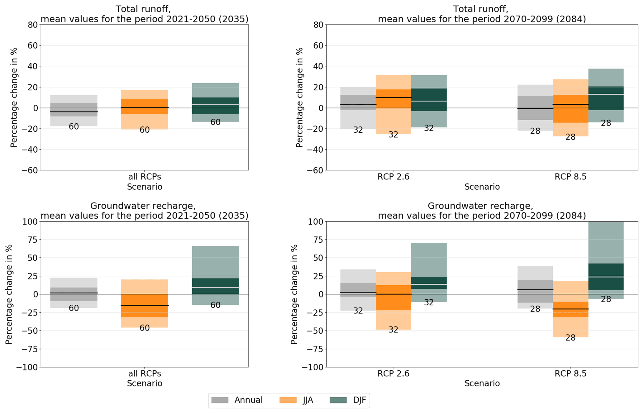
Figure 5Percentile boxes showing the potential percentage changes in the mean total runoff and mean groundwater recharge of the multi-model ensemble in the periods around 2035 (2021–2050) and 2084 (2070–2099) relative to the reference period around 1985 (1971–2000) in the BRR. The figure shows the annual and seasonal (summer months of June, July, and August (JJA) and winter months of December, January, and February (DJF)) means. For the period around 2084, the results are shown separately for the emission scenarios RCP 2.6 and 8.5. In the period around 2035, the simulations of both emissions scenarios RCP 2.6 and 8.5 are shown together in one percentile box (“all RCPs”). The black numbers below the percentile boxes show the number of model combinations of the multi-model ensemble. For groundwater recharge in winter months under RCP 8.5 in the period around 2084, the percentile box was cut for better visualization as its P90 lies at around 150 % (see Fig. 1). This figure was shown to the stakeholders directly after Fig. 4 and was explained as shown in “Communication of potential changes in 30-year mean values by percentile boxes”. An interpretation of the results is given in Appendix A10.
When presenting the project results after the participatory process, we also first explained why and how we quantified the uncertain future hydrological changes with the slide in Fig. 3. Then, the potential changes in the 30-year mean values were communicated by percentile boxes (with the same approach as in the first workshop; see “Communication of potential changes in 30-year mean values by percentile boxes”), and, finally, an alternative communication of potential changes in 30-year mean values by tables was used to be compared to our communication approach by percentile boxes (see “Alternative communication of potential changes in 30-year mean values by tables”).
Communication of potential changes in 30-year mean values by percentile boxes
To show potential changes in 30-year mean values, we designed percentile boxes (Sect. 2). Percentile boxes are similar to boxplots but are easier to understand because they avoid the boxplot whiskers (Sect. 1). We selected five characteristic percentiles of the multi-model ensemble output to inform stakeholders about potential future changes in both total runoff and groundwater recharge. The characteristic values P10, P30, P50 (median), P70, and P90 represent the interpolated values of percent change in either total runoff or groundwater recharge that are not exceeded by 10 %, 30 %, 50 %, 70 %, and 90 % of the 32 (or 28 or 60) values of the multi-model ensemble, respectively.
P10 and P90 form the outer margins of the percentile box, P30 and P70 are the margins of the darker box inside the whole percentile box, and P50 (the median) is displayed as a line within the percentile box (Fig. 4). Thus, the projected changes in 80 % of all ensemble members are represented by the percentile box; the number at the bottom of the percentile box shows the number of model combinations in the multi-model ensemble. When informing about potential changes in 30-year mean values in the first workshop, we first explained the percentile boxes with the characteristic values while showing Fig. 4.
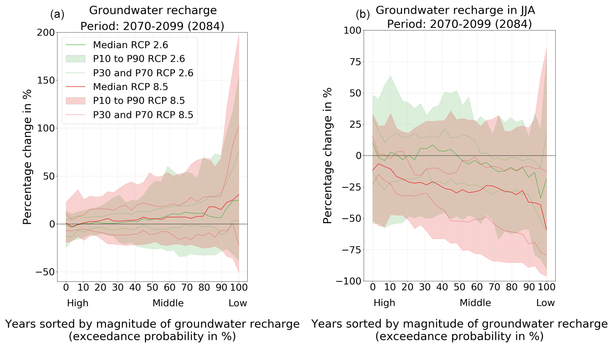
Figure 6The third diagram, which was explained to the stakeholders in the first workshop, shows changes in the interannual variability of groundwater recharge. Percentage change in annual groundwater recharge (a) and summer groundwater recharge in June, July, and August (JJA; (b)) in the period around 2084 (2070–2099) relative to the reference period around 1985 (1971–2000) in the BRR. The 30 yearly groundwater recharge values are sorted according to their magnitude, and the relative changes were calculated between the values of the same rank in the future and reference periods. This sorting corresponds to the exceedance probability, which is shown in percent. As an example, an exceedance probability of 90 % in the left diagram refers to the year in which groundwater recharge is lower than in 90 % of all years, i.e., lower than in 27 out of 30 years. If the percentage change for this unusually dry year is −10 %, this means that the model projects that the groundwater recharge that is exceeded only in 3 out of 30 years in the future is 10 % lower than in the respective year of the reference period. This figure was shown to the stakeholders directly after Fig. 5 and was explained as shown in “Communication of potential changes in interannual variability”. An interpretation of the results is given in Appendix A11.
After communicating how and why we quantified the hydrological hazard indicators with their uncertainty (Fig. 3) and the percentile box (Fig. 4), we presented the quantification results. We clarified how the visualization can be interpreted first with the results of the potential changes in 30-year mean values with their uncertainty, as shown in Fig. 5. As an example, we explained the potential change in groundwater recharge in the period 2070–2099 (see the lower-right diagram in Fig. 5) in the following way.
For the annual mean values, the dark-gray box is never completely above or below 0 %, and the median lies near 0 %. This means that about 50 % of the multi-model ensemble estimates a decrease, and about 50 % estimates an increase. In the summer and winter months, you can see a better tendency: the dark-green box of the winter months is completely above 0 %. This means that at least 70 % of the multi-model ensemble estimates an increase in the winter months. For the summer months (under RCP 8.5), at least 70 % of the multi-model ensemble estimates a decrease because the dark-orange box lies completely below the 0 % line. This indicates a potential hazard for, e.g., the drinking-water supply in summer months in the future. Furthermore, 10 % of model combinations even project a decrease in summer groundwater recharge by more than 60 %.
We pointed out that none of the percentile boxes are completely above or below 0 %. This means that in no examined case did 90 % or more of the multi-model ensemble agree on the direction of change.
Communication of potential changes in interannual variability
We also displayed the course of the five characteristic values over the sorted means (exceedance probabilities) of total runoff and groundwater recharge of each year in the two future periods. This shows the probability and uncertainty of changes in interannual variability, in particular how statistical dry years, with, e.g., very low groundwater recharge, may change in the future as compared to statistical wet years. We displayed the changes in groundwater recharge in wetter to drier years in a “continuous percentile box”. Two examples of a continuous percentile box were shown to the stakeholders in the first workshop and are shown in Fig. 6, where the x axis indicates the exceedance probability of annual and summer groundwater recharge. For example, a value of 90 % on the x axis represents the annual or summer groundwater recharge in a rather dry year, a year with an annual or summer recharge that is exceeded in 90 % of the 30 years of the reference and future periods. The y axis shows the percentage change in the annual or summer groundwater recharge between the reference period and the future period (2077–2099). We told the stakeholders how they could relate the solid and dashed lines and the margins of a colored area in Fig. 6 to the percentile boxes of Fig. 5 shown before.
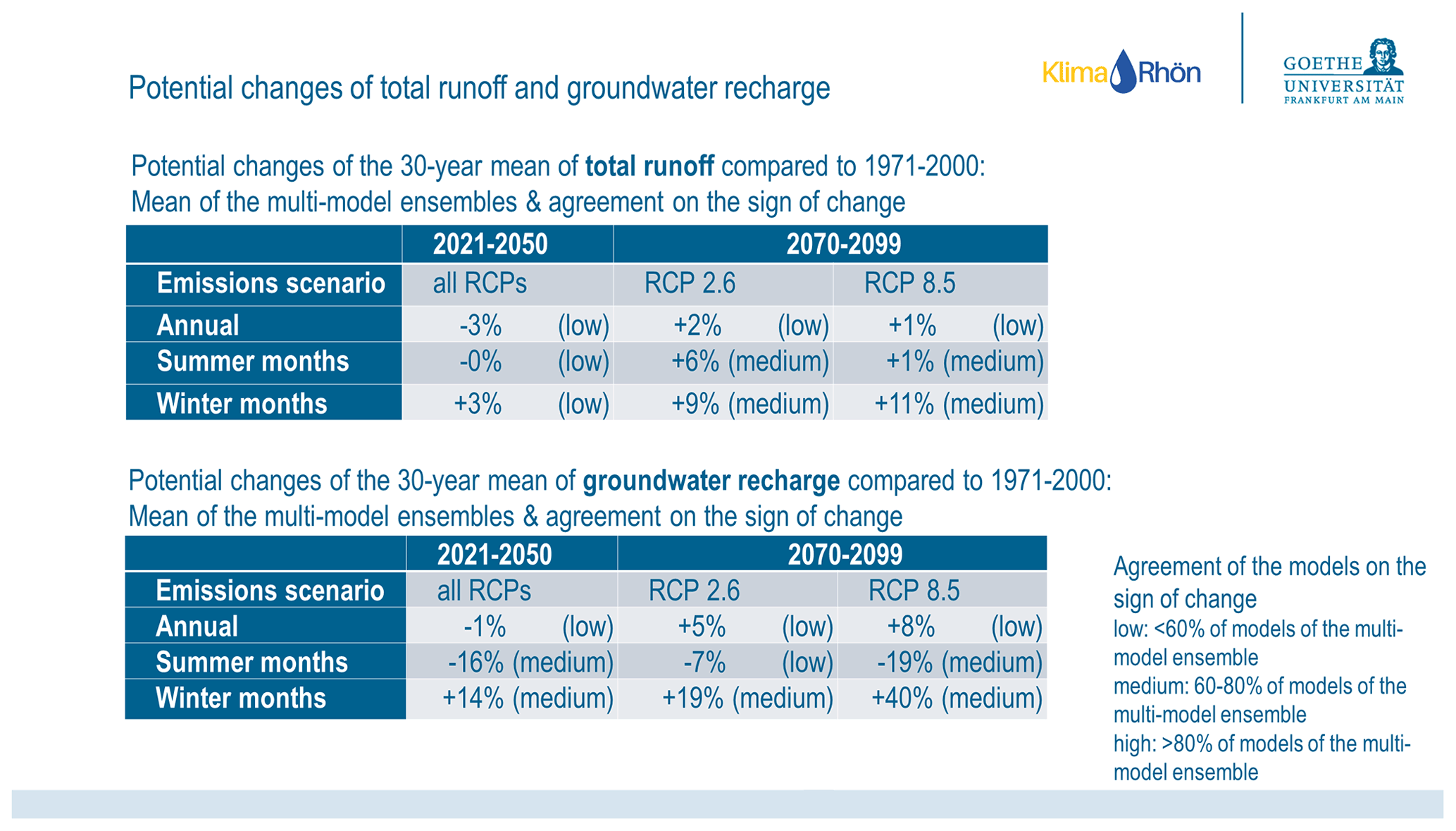
Figure 7With this slide (the original slide was in German) we show the change in mean total runoff and mean groundwater recharge in the periods 2021–2050 (2035) and 2070–2099 (2084) as compared to 1971–2000 for the whole year (annual); only the summer months and only the winter months were shown in an alternative way as compared to the percentile boxes (Fig. 5). For the period 2070–2099, the results are shown separately for the emissions scenarios RCP 2.6 and 8.5. In the period 2021–2050, the simulations of both emissions scenarios RCP 2.6 and 8.5 are shown together in one column (“all RCPs”). Agreement within the multi-model ensemble on the sign of change is provided in parentheses: in the case of low model agreement, < 60 % of models agree on the sign of change; in the case of medium model agreement, 60 %–80 % of models agree on the sign of change; in the case of high model agreement, > 80 % of models agree on the sign of change. This slide was not shown to the stakeholders in the first workshop of the participatory process. The left logo in the top-right part was created by Max Czymai.
In the first workshop, after presenting the potential changes in 30-year mean values with their uncertainty (Fig. 5), we explained the continuous percentile box with the characteristic values and then communicated the potential changes in interannual variability. We showed the changes in the interannual variability of groundwater recharge averaged over (1) all months (Fig. 6a) and (2) only the summer months (Fig. 6b) in the years of the period 2070–2099 to the stakeholders because we assumed the demand for adaptation in water management for groundwater recharge in the summer months to be higher than in the winter months after the stakeholder interviews. As an example, we explained the potential change in the mean summer groundwater recharge in the period 2070–2099 (Fig. 6b) in the following way.
Here, in summer, let's focus on RCP 2.6 (green). The median drops to the right – on the right are drier years! In wetter years (on the left), the median lies near 0 %. So, about 50 % of the multi-model ensemble estimates a decrease, and about 50 % estimates an increase in wetter years. In drier years (on the right), you can see that even P70 – the upper dashed line – drops below 0 %. This means that 70 % of the multi-model ensemble estimates a decrease in summer months in drier years. Here, you see a difference in the consensus of the multi-model ensemble in terms of the direction of potential changes between wetter and drier years. In drier years, the likelihood of an emerging hazard (less groundwater recharge in summer months than historically) is higher than in wetter years.
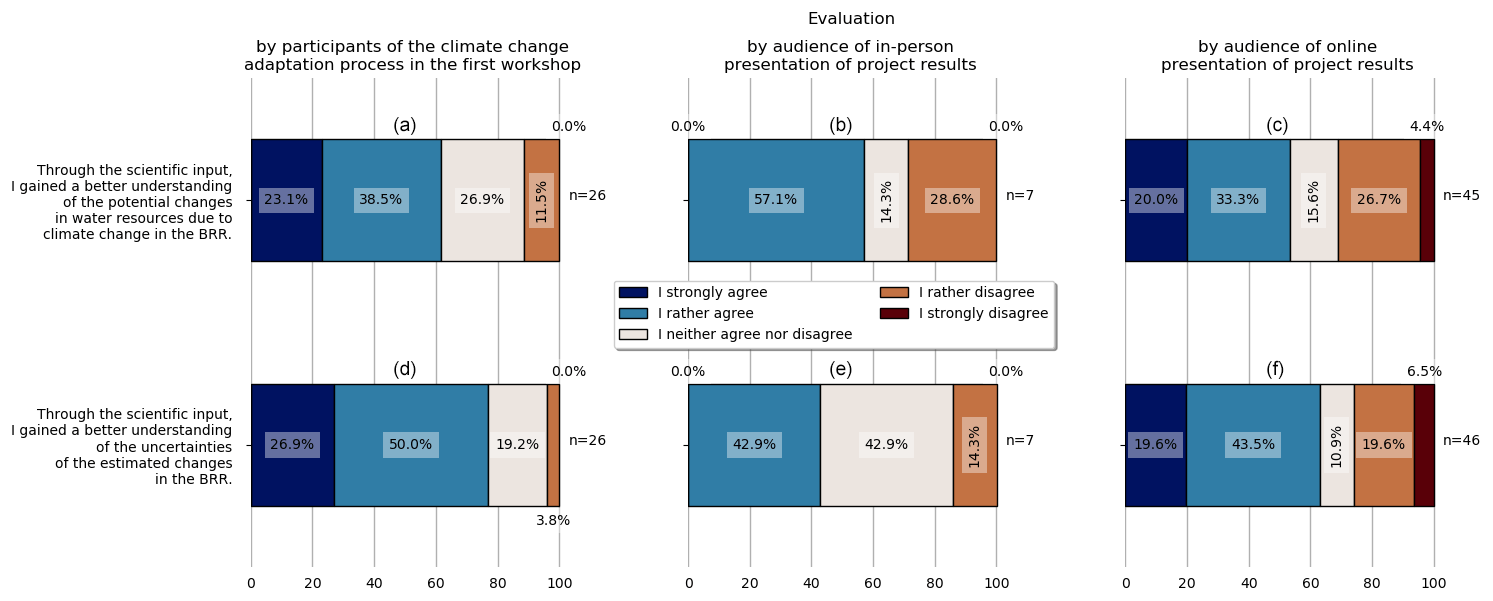
Figure 8Results of the evaluation of the scientific input in the first workshop of the participatory process (a, d) and in the in-person presentation (b, e) and online presentation (c, f) outside of the participatory process. The stakeholders and the audiences of the project presentations rated their agreement on the statements “Through the scientific input/the results (figures) just presented, I gained a better understanding of the potential changes in water resources due to climate change in the biosphere reserve Rhön” (a, b, c) and “Through the scientific input/the results (figures), I gained a better understanding of the uncertainties of the estimated changes in the biosphere reserve Rhön” (d, e, f). The bars show the results of the answers of 26 stakeholders (a, d), 7 participants (b, e), and 45 and 46 participants (c, f). BRR: UNESCO biosphere reserve Rhön.
Summarizing hazards for the stakeholder discussion
After the presentation of the potential changes in the 30-year mean values and the interannual variability, along with their uncertainty, in the plenary, we organized a World Café. On one of the tables, all the stakeholders discussed, for about 15 min, the following question: “What future climate-change-driven changes in groundwater recharge and runoff, which can only be estimated with uncertainty, do we want to prepare for?” This was to determine the risk aversion or affinity of the stakeholders. To support the discussion, summarizing the multi-model results shown in the plenary, we showed the following information at the World Café table:
-
Potential change in mean annual total runoff amounts to −20 % to +20 %, with a median near 0 %.
-
Potential change in mean annual groundwater recharge amounts to −25 % to +25 %, with a median near 0 %.
-
Potential change in mean groundwater recharge in summer months (June, July, August) amounts to −70 % to +25 %, with a median at approximately −20 %; groundwater recharge declines particularly sharply in dry years.
The ranges correspond approximately to the P10 and P90 values. We did not present stakeholders with the lowest value, i.e., the strongest simulated decrease in the multi-model ensemble. The worst-case scenario, which we presented, included percentage reductions that are exceeded by only 10 % of the multi-model ensemble, representing the smallest values within the three ranges mentioned above.
Alternative communication of potential changes in 30-year mean values by tables
The tables shown in Fig. 7 were presented to the audiences of the two presentations of project results (outside of the participatory process) to compare our visualization format (see “Communication of potential changes in 30-year mean values by percentile boxes”) with this alternative communication format. The tables represent the same data on future groundwater recharge and runoff changes that are shown by the percentile boxes (Fig. 5) in an alternative, simpler, and more common format, in the form of a table with numerical values, the mean change in the ensemble members, and verbal expressions describing the agreement of the ensemble members on the sign of change. If more than 80 % of models agreed on the sign of change, we assigned high agreement. If 60 %–80 % of models agreed on the sign of change, we assigned medium agreement, and if less than 60 % of models agreed on the sign of change, we assigned low agreement.
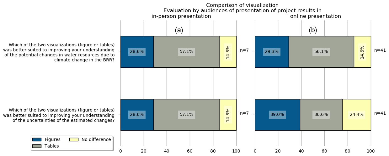
Figure 9Comparison of visualization formats in the in-person presentation (a) and the online presentation (b) of project results outside of the participatory process. The bars show the results of the answers of 7 and 41 participants. BRR: UNESCO biosphere reserve Rhön.
4.1 Interpretation of communicated hazard indicators by the stakeholders
In the discussion about what degree of changes the BRR should aim to adapt to (see “Summarizing hazards for the stakeholder discussion”), all except one advocated for adapting to the worst case (the strongest decreases presented were P10), driven by the precautionary principle and the recognition of the time required for practice adjustments. These reductions include groundwater recharge decreases of over 70 % in summer and annual groundwater recharge decreases of 25 %. However, concerns were raised regarding the potential cost and frustration associated with preparing for worst-case scenarios that might not materialize. Another stakeholder asked herself how important it is to decide to adapt to a specific (i.e., deterministic) potential change, arguing that a wrong certainty was conveyed if they decided to adapt to a specific potential change. On the other side, it was discussed that, for some (technical) adaptation measures, a specified quantity of potential change is needed. Moreover, they highlighted the limitations of mean annual total runoff as an informative indicator and instead emphasized the importance of focusing on extreme events. In summary, the need for anticipatory, flexible, and robust measures in response to uncertainties was stressed, with stakeholders being very risk-averse. The presentation of potential future groundwater recharge changes in summer months, along with the stakeholders' experiences of unusually dry years, particularly in summers, in the study area and across Germany before and during the participatory process, led to a focus on adapting to potential water scarcity in summer months.
4.2 Evaluation of the communication format by the stakeholders of the KlimaRhön participatory process
At the end of the first workshop, the stakeholders anonymously evaluated the applied methods for embracing uncertainty (the evaluation data can be found in Müller and Czymai, 2022). The stakeholders were asked to rate their agreement on the statement “Through the scientific input, I gained a better understanding of the potential changes to water resources due to climate change in the biosphere reserve Rhön”. The scientific input consisted of the explanation and discussion of simulated mean and interannual changes in total runoff and groundwater recharge as presented in “Communication of potential changes in 30-year mean values by percentile boxes”, “Communication of potential changes in interannual variability”, and “Summarizing hazards for the stakeholder discussion”. For more than 60 % of the 26 stakeholders, the scientific input enhanced the understanding of potential changes in water resources, while 12 % of stakeholders rather disagreed with the statement, and no stakeholder strongly disagreed (Fig. 8a). Even more than 75 % of the stakeholders strongly agreed or rather agreed with the statement “Through the scientific input, I gained a better understanding of the uncertainties of the estimated changes in the biosphere reserve Rhön” (Fig. 8d). Only one stakeholder rather disagreed with the statement, and none strongly disagreed.
4.3 Comparison of our communication format with a more common communication format by the audiences of two presentations of the project results
To compare the communication format of potential hydrological changes – more precisely of changes in 30-year mean values – by means of percentile boxes (Fig. 5) with a more common communication format (Fig. 7), we used the opportunity of two presentations, in which we presented the outcomes of the project KlimaRhön at the end of the project (June and July 2023; Sect. 3.2.1; the questionnaire can be found in Sect. S2 in the Supplement). In each of the two presentations, we first presented the potential future changes in mean groundwater recharge and runoff in the same manner as in the first workshop of the participatory climate change adaptation process, described in “Communication of potential changes in 30-year mean values by percentile boxes”. Directly afterward, we asked the audience to anonymously rate their agreement with the same two statements rated by the KlimaRhön stakeholders in the first workshop of the participatory process. For the first statement, “Through the results (figures) just presented, I gained a better understanding of the potential changes in water resources due to climate change in the biosphere reserve Rhön”, only 57 % of the audience of the in-person presentation rather agreed, while 28 % rather disagreed (no one strongly agreed or strongly disagreed; Fig. 8b). On the other hand, 53 % of the audience of the online presentation strongly or rather agreed with the first statement, while 31 % strongly or rather disagreed (Fig. 8c). For the second statement, “Through the results (figures) just presented, I gained a better understanding of the uncertainties of the estimated changes in the biosphere reserve Rhön”, 43 % of the audience of the in-person presentation rather agreed, while 14 % rather disagreed (Fig. 8e). On the other hand, 63 % of the audience of the online presentation strongly or rather agreed with the statement (Fig. 8f). Like in the first workshop of the participatory process, more participants of the online presentation agreed that they had gained a better understanding of the uncertainties more so than having gained a better understanding of the potential changes (Fig. 8c and f). The evaluations of our communication format by percentile boxes differ between the groups (stakeholders in the workshop, audience in the in-person presentation and audience in the online presentation) because the evaluation in the workshop of the participatory process was conducted after the stakeholders were also shown the interannual variability changes (Fig. 6), summarized multi-model results (see “Summarizing hazards for the stakeholder discussion”), and then had time to discuss the potential hydrological changes in the World Café (Sect. 4.1), while the evaluations in the two presentations were conducted directly after communicating the 30-year mean values with their uncertainty. In addition, the participant composition of the groups was very different.
Directly after this evaluation (Fig. 8b–c and e–f), the tables shown in Fig. 7 were presented to the audiences of the two presentations. Then, we asked the audiences to anonymously indicate which of the two visualizations was better suited to improving their understanding of the potential changes and their uncertainties, the percentile box figure (Fig. 5) or the tables (Fig. 7). For the first question, “Which of the two visualizations (figure or tables) was better suited to improving your understanding of the potential changes in water resources due to climate change in the BRR?”, and the second question, “Which of the two visualizations (figure or tables) was better suited to improving your understanding of the uncertainties of the estimated changes?”, 57 % of the seven participants of the in-person presentation preferred the tables, and only 28 % preferred the percentile box (Fig. 9a). Similarly, 56 % of 41 participants in the online presentation preferred the table, and 29 % preferred the percentile boxes for improving their understanding of the potential changes (Fig. 9b upper bar). However, for the second question on understanding the uncertainties, only 37 % of the audience of the online presentation preferred the tables, and 39 % preferred the percentile boxes (Fig. 9b lower bar).
5.1 Why and how should the uncertainty of hydrological changes due to climate change be quantified with a multi-model ensemble of global models?
Uncertainty of future climate change hazards is expected to be high due to the complexity of the Earth system and human decision-making, highlighting the need to embrace uncertainty and to work on reducing the uncertainty of projected climate change and the related hazards (Mearns, 2010). Both global climate models and global hydrological models have a low spatial resolution and do not consider the high spatial heterogeneity that can be important for local-scale adaptation to climate change. Higher-resolution modeling efforts, if restricted to one local hydrological model, might be better suited for simulating the historic development in a study region but are expected to lead to an underestimation of uncertainty regarding future changes. One reason is that the (again uncertain) impact of adapting vegetation on water resources (Reinecke et al., 2021) is mostly not taken into account by hydrological models. Therefore, we suggest using, under most circumstances, the available multi-model ensemble output of the ISIMIP initiative to quantify potential future changes in physical variables and their uncertainty, in a similar fashion to what we did in the presented case study, and not using a single local or regional impact model. A multi-model ensemble including regional models (combinations of regional climate and regional impact models or global climate and regional impact models) would be favored over a multi-model ensemble of only global models. While the coarse resolution of the global multi-model ensembles of the ISIMIP initiative certainly leads to increased and non-quantifiable uncertainty, a major advantage is its usability for participatory climate change adaptation processes worldwide. We found that, even with the coarse resolution of the results, they helped the stakeholders to understand future water-related hazards of climate change and their uncertainty in the study regions and, based on this, to focus their search for adaptation measures. However, quantifying the potential changes needs an expert with basic technical knowledge in any programming language.
We considered the three complementary paradigms for modeling the future by Maier et al. (2016): anticipation of the future was done by the GCMs and GHMs used, (approximate) quantification of future uncertainty was achieved using multi-model ensembles, and the exploration of multiple plausible futures was done using two emissions scenarios.
The monthly time series of a large number of hydrological variables that are provided in ISIMIP should be used to compute hazard indicators that are most relevant for the climate change risks of interest. For example, while groundwater recharge (renewable groundwater resources) is a fraction of total runoff (renewable water resources), the change in mean groundwater recharge differs appreciably from projections of total runoff, particularly in the summer months; thus, it is better to analyze groundwater recharge projections if groundwater is important for human water supply. Changes in variability and extremes should also be analyzed specifically as it is generally assumed that climate change changes variability and thus, e.g., drought and floods. Additional hazard indicators should be analyzed after major risks have been identified together with stakeholders based on the vulnerabilities of the system of risk. This may also include different spatial and temporal aggregations of the multi-model ensemble output, e.g., regarding seasons.
Results of multi-model ensembles may underestimate the uncertainty, which was shown with an initial-condition large ensemble by Mankin et al. (2020). This initial-condition large ensemble consisted of seven climate models which were run with different initial conditions and simulated a larger uncertainty range than CMIP5, an ensemble of 40 climate models. Such initial-condition large ensembles, however, are not sufficiently feasible, especially for climate change impact studies, because of the large computational resources required to run the model combinations (as in the example of Mankin et al., 2020: 286 climate model runs, which would then be multiplied by the number of impact models). Moreover, the initial-condition large ensemble would also need to embrace parameter uncertainty, which would increase the model runs.
5.2 How can the uncertainty of hydrological changes due to climate change be best communicated?
Visualization of uncertainty by percentile boxes enables stakeholders to read the change values they wish to adapt to, depending on the problem (resource scarcity vs. resource excess) and their risk aversion (low vs. high). For example, a stakeholder with a high risk aversion towards reduced water availability can choose P10 of the 30-year mean change in summer months (from the percentile boxes of Fig. 5) or even P10 in summer months for statistical dry years with an exceedance probability of 90 % (continuous percentile box of Fig. 6) under the emissions scenario RCP 8.5. With our proposed types of visualization, percentile box, and continuous percentile box, stakeholders should be empowered to recognize the uncertainty and probability of potential changes for, on the one hand, a future period on average and, on the other hand, for years with different water availability in a future period. However, the communication, i.e., the explanation of the approach and the interpretation, requires a considerable amount of time in a workshop and asks the stakeholders for a long concentration span. To further increase the information content of percentile boxes, the numerical value of the change at each of the five percentiles could be written on or next to the respective line, which, however, would require larger percentile boxes. The visualization of changes in interannual variability by the continuous percentile box remains rather difficult to understand and requires, for most stakeholders, a longer exposure than was possible during the workshop. In addition, for Fig. 6, we would propose changing the colors to such that are more visible to persons with color vision deficiency and thickening the lines of the inner percentiles for better visibility.
To avoid the wrong interpretation that the percentiles reflect true probabilities of occurrence (while they are only a very rough approximation of probabilities; Döll et al., 2015), we did not use the wording “with a probability of”, also following Jack et al. (2020). The hazard uncertainty was suitably communicated in the participatory KlimaRhön process by always referring to the fraction of the ensemble members that project changes of less or more than a certain value. By using the fraction of the ensemble members instead of terms like “the majority” or “most of the models”, we may have prevented subjective misinterpretation of the actual fraction. For instance, some individuals might perceive 60 % as “the majority”, whereas some scientists consider 90 % to 100 % to be representative of a consensus (van der Bles et al., 2019). In addition, the communication of potential changes in groundwater recharge and total runoff might be more effective when they are related qualitatively to possible impacts and the reality of the life of the stakeholders (Corner et al., 2018). We suggest giving examples of the potential impacts connected to the indicated hazards, e.g., the impacts of reduced summer groundwater recharge on drinking-water supply or on the discharge of springs with related ecological impacts, and showing illustrative images (e.g., from https://climatevisuals.org/, last access: 16 May 2024; Corner et al., 2018).
The stakeholders and the audience of the online presentation rated their enhanced understanding of the potential changes somewhat lower than their enhanced understanding of uncertainty (Fig. 8). This might be due to the large uncertainties and the fact that the multi-model ensemble of potential changes never fully agreed on the direction of change. Comparing our communication of potential changes in 30-year mean values by means of percentile boxes (see “Communication of potential changes of 30-year mean values by percentile boxes”) with a more common communication of the means of the multi-model ensembles in tables (see “Alternative communication of potential changes of 30-year mean values by tables”), the audiences in the in-person and the online presentation preferred the more common visualization (tables) for an enhanced understanding of the potential hydrological changes. However, for improving their understanding of the uncertainties of these potential changes, an additional 20 % found the figures to be more suitable or equally as suitable as the tables compared to improving their understanding of the potential changes themselves (Fig. 9). Of that 20 %, half preferred our communication format with the figure; i.e., they find that the more common communication with the tables helped to understand the potential hydrological changes but did not adequately account for uncertainties. The other half is undecided on whether the figure or the tables are more suitable for uncertainty communication. Possibly, our communication with the percentile boxes did not fit with the data normally used by the participants (lack of interplay; Lemos et al., 2012) or their (work) experience (tacit knowledge; Höllermann and Evers, 2019). We suspect that participants might have preferred the percentile boxes if (1) they had more time to interpret them and (2) they needed to use the hazard information for defining adaptation measures. We believe that our approach for communicating uncertainties in the stakeholder workshop of the participatory process was suitable and at an appropriate level of complexity, also because more than 75 % of the stakeholders and 63.1 % of the audience in the online presentation (Fig. 8) agreed to have gained an enhanced understanding of the uncertainties. However, it must also be mentioned that this positive evaluation regarding their better understanding of uncertainties might have also been caused by a bias. They might have either wanted to give “socially wanted answers, or [they] might [have wanted] to give themselves the idea that their time was well spent” (Kok and van Vliet, 2011, p. 102).
To tackle uncertainty, practitioners already have different routines but usually do not analyze model ensembles and their uncertainty themselves (Höllermann and Evers, 2019). By showing the stakeholders the uncertainty of the models through multi-model ensembles and showing them the approach of our quantification, we address one of the uncertainty routines of stakeholders called “transparency”, in which the stakeholder considers the limits of knowledge (Höllermann and Evers, 2019). Moreover, decision-makers have to perceive the information as accurate, credible, salient, timely, and useful for the decision-making need, and they should not perceive it as risky to use the information (Lemos et al., 2012). Cash et al. (2002) found that the critical determinants of information for decision-making are credibility, salience, and legitimacy, of which all must be fulfilled, but that decision-makers (or, in general, audiences) differently perceive and value these attributes. We think that we made the simulation results more credible and salient and as low risk as possible by showing uncertainty with the results of a multi-model ensemble in the percentile boxes and explaining them.
5.3 Evaluations in participatory processes
A research gap exists on how to best evaluate participatory methods (Lange et al., 2021; Rosener, 1981). The evaluation conducted in this study is only a weak form of evaluation because of the small number of evaluating participants and the high context dependence, as is often the case in participatory processes. In participatory processes, no controlled experiments are possible due to the nature of participatory processes and ethical reasons (Lange et al., 2021). In addition, it is not practicable or even possible to form two groups subjected to “alternative treatments”, such as in, e.g., clinical studies. This would require organizing two parallel time-consuming participatory processes. We did not want to disturb the participatory process and burden the stakeholders with scientific investigations; hence, we used the opportunity of the two presentations of project results after the end of the participatory process for a comparative evaluation. This evaluation was not done by presenting each of the two communication formats to a different group as we could not expect that the audiences would be comparable; instead, the two formats were presented and evaluated one after the other. However, the evaluation is only a weak evaluation in the sense that it did not evaluate the formats in the context of a participatory process on climate change adaptation but within a presentation of project results. Even in participatory adaptation processes, the participants' expectations and needs for information differ (Rosener, 1981). In general, we can distinguish the information needs of stakeholders that need to identify adaptation measures in response to the presented climate change hazards from the information needs of audiences of a presentation of project results. In the workshop, the hydrological changes due to climate change, along with their uncertainties (Figs. 5 and 6), were communicated to the stakeholders to support their development of adaptation measures, which was evident to the stakeholders when listening to the scientific input. The audiences of the presentations did not have to develop adaptation measures; therefore, a less detailed and thus simpler communication format (Fig. 7) than the percentile box (Fig. 5) was sufficient, but this would not be sufficient as a basis for identifying adaptation measures. Moreover, the time that the stakeholders dealt with the information at the workshop was much longer. The evaluation in the workshop was conducted only after the stakeholders were also shown the interannual variability (Fig. 6) and the most important hydrological change ranges (see “Summarizing hazards for the stakeholder discussion”) and then had time to discuss the potential hydrological changes in the World Café (Sect. 4.1), while the evaluations in the two presentations were conducted directly after communicating the 30-year mean values, along with their uncertainty, with the two communication methods. Therefore, the comparative evaluation of the two communication formats by the audiences of the presentations is not relevant for the communication format in participatory climate change adaptation processes.
5.4 Using the uncertain information about future climate change hazards for the development of adaptation measures
The stakeholders in the first KlimaRhön workshop expressed a preference for following the precautionary principle and wanted to adapt to a worst-case scenario regarding water scarcity in the summer months (a strong decrease in groundwater recharge) rather than to an increase in groundwater recharge, even though this was within the simulated ensemble range, with the median being close to zero. At this early point, they did not see the need to agree on adapting to a specific future change in groundwater recharge (Sect. 4.1) because adaptation measures were only generally discussed. The specific results of the multi-model ensemble were not used quantitatively (only qualitatively) in the discussion of adaptation measures because no technical measures (e.g., well drilling and networking of pipelines) that must be based on a specific decrease in groundwater recharge were planned, and no monetary cost–benefit analyses were performed in the participatory process. With our percentile boxes, decision-makers can use the provided range of potential changes in, e.g., exploratory modeling to stress test the system with different plausible futures and possible decisions, which would not be possible with the results in the more common communication format (Fig. 7).
Communicating and embracing uncertainty is important “to help policy-makers and practitioners make the best possible decisions, which cannot be based on the available evidence alone. […] [T]aking unknowns into account aims to allow more realistic assessment of the adequacy of decisions, as well as better preparation for things that can go wrong” (Bammer, 2013, p. 64). Due to highlighting the uncertainty of future changes, we hope that the stakeholders will more carefully embrace uncertainty in their decision-making in the future. Next to the uncertainty of climate change hazards (comprising the climate and hydrological model uncertainty and the uncertainty of greenhouse gas concentrations), the uncertainty of suitable adaptation measures, i.e., uncertain transformation knowledge (Becker, 2002), persists as multiple plausible futures could unfold. This uncertainty should be embraced, e.g., with participatory scenario development (Carlsson-Kanyama et al., 2008; Maier et al., 2016; Döll and Romero-Lankao, 2017; Voinov et al., 2018), ensuring stakeholders are not overwhelmed by the level of uncertainty (Jack et al., 2020). These scenario developments usually produce explorative or normative scenarios (Table A1) and need the (uncertain) climate change information as boundary conditions. To support local climate change adaptation, distributions of potential future climate change hazards from global-scale multi-model ensembles can be integrated with local data in Bayesian networks that represent the causalities of, e.g., local water scarcity (Kneier et al., 2023). Then, adaptation strategies should be developed that work under multiple plausible futures, i.e., which are more robust and adaptive (Maier et al., 2016), and incorporate the acceptance of the relevant actors to implement the adaptation measure(s). In the KlimaRhön project, this was done in the workshops that followed the first workshop, in which the climate change hazards to which the stakeholders wanted to adapt were identified.
With ongoing climate change, adaptation to climate change has to happen everywhere around the globe at local to regional scales. Adaptation measures should be identified in participatory processes involving local stakeholders and professionals with a scientific background by embracing the multiple uncertainties that affect the future success of adaptation measures. In this study, we present a readily applicable approach for quantifying and communicating climate change hazards and their uncertainties with multi-model ensembles. This approach is applicable in many climate change adaptation processes worldwide; it is not restricted to hydrological hazards but can also be used in climate change adaptation processes in the fields of agriculture, forestry, fisheries, and biodiversity.
The presented method for producing quantitative estimates of future climate change hazards, which benefits from the freely available output of global multi-model ensembles (provided by the ISIMIP initiative), can be replicated by anybody with basic knowledge in any programming language such as R, Python, or MATLAB. Due to the high uncertainty of the translation of climatic changes into hydrological changes, utilization of the multi-model ensemble output is preferable, even for local study areas, unless multiple local hydrological models are available; with only one hydrological model, the uncertainty of future changes would be underestimated. We recommend quantifying hazards as relative changes as these can be estimated more robustly by multi-model ensembles than by absolute values or changes in absolute values. Based on the questionnaire-based evaluations of the participants, we can conclude that different formats for communicating the range of potential future changes should be used when addressing either the stakeholders in a climate change adaptation process or the general public. Stakeholders who need to identify adaptation measures based on uncertain future hazards are best informed about the hazards by percentile boxes that show which relative change of a variable is exceeded according to which percent of all ensemble members. Distinguishing five percentiles in an easy-to-grasp visualization with an appropriate degree of complexity, percentile boxes enable the stakeholder to select which future changes they plan to adapt to, depending on their risk aversion. For the presentation of climate change hazards to the general public, a simple table with the mean changes and an indication of the agreement of the models on the sign of change is preferable. Communicators should always reflect upon and decide what information should be the focus of a visualization.
When presenting climate change hazards, we propose communicating what share of the multi-model ensemble simulates a change instead of stating this share of the multi-model ensemble as a probability. This communication approach avoids the uncertain relation of ensemble percentiles to probabilities and moves the multi-model ensemble from a shallow to a shallow-medium uncertainty level. We suggest that an improved visualization and communication format for the important changes in interannual variability be investigated in the future.
However, as legitimacy, credibility, and salience are perceived differently by individual stakeholders, no perfect, standard method to communicate information can be identified; “our worldviews, values, and social norms dictate how we receive information and apply it” (Corner et al., 2018, p. 3). A potential remedy is to implement cultural theory into the communication strategy, which categorizes people into four cultural worldviews when dealing with risks: hierarchists prefer expert opinions and regulations; egalitarians value societal contributions for risk reduction; individualists prefer market-based solutions; and fatalists are apathetic, viewing risks as unpredictable and random (Verweij et al., 2006; Czymai, 2023). These cultural worldviews could be integrated into the communication strategy to convince a heterogeneous audience to embrace uncertainty in their decision-making, and the impact should be evaluated. To address hierarchists, it could be communicated that practitioners and scientists view uncertainty information as relevant (Höllermann and Evers, 2017). For egalitarians, it could be communicated that embracing uncertainty promotes fairness and prevents exposing only a few individuals to hazards due to collective inaction. Individualists could be approached by elucidating that embracing uncertainty could maintain their capacity to act and foster innovation.
Despite the coarse model resolution and wide uncertainty ranges, the multi-model ensemble results and their suitable communication helped the stakeholders in the participatory KlimaRhön process to understand uncertainty and to develop robust and flexible adaptation options. With our approach to quantifying and communicating multi-model ensemble results as a basis, flexible climate change risk management strategies can be developed jointly by stakeholders and scientists in a participatory and transdisciplinary manner.
A1 Impact models
Quantification of the potential future changes in relevant characteristics of the physical system, such as groundwater recharge or agricultural yield, is achieved by analyzing either the output of climate models or the output of impact models that are driven by the output of climate models. Impact models are domain-specific models, such as hydrological models or crop models, that focus on the simulation of certain subsystems of the Earth system. Analysis of impact model output is preferred when climate models do not compute the variable of interest or when impact models are assumed to provide a better representation of reality, e.g., due to the spatial scale or the bias of climate model output. Due to the low accuracy of climate models when simulating current climate conditions, climate model output is first bias-adjusted using historic climate data before it is applied to drive impact models (Frieler et al., 2017).
A2 Multi-model ensemble
The multi-model ensemble of the study consists of 32 model combinations of four global climate models and eight global hydrological models, which took part in the ISIMIP2b project. The four global climate models are IPSL-CM5A-LR, GFDL-ESM2m, MIROC5, and HadGEM2-ES. The eight global hydrological models that were used are CLM4.5, CWatM, H08, JULES-W1, LPJmL, MATSIRO, PCR-GLOBWB, and WaterGAP2. The ISIMIP2b project prescribed in its protocol (ISIMIP, 2019) that the models should be run with different climate and CO2 concentration scenarios and socio-economic scenarios. For the future periods, we used the model output of the CO2 concentration scenarios “rcp26” and “rcp85”, each with the socio-economic scenario “2005soc”. For the reference period, we used the socio-economic scenario “histsoc” with the CO2 concentration scenario “historical”.
However, some models cannot execute some of these runs. The global hydrological model PCR-GLOBWB was not run for the climate and CO2 concentration scenario “rcp85”, which is why the multi-model ensemble only consists of 28 model combinations for the scenario “rcp85”. Moreover, the hydrological model CLM4.5 was not run with the socio-economic scenario “histsoc” but with the socio-economic scenario “2005soc” in the reference period, and the global hydrological model JULES-W1 is not run with any of the previously mentioned socio-economic scenarios but with the scenario “nosoc”.
A3 ISIMIP
ISIMIP developed a protocol with which international global hydrological modeling groups consistently executed the simulations (Frieler et al., 2017), resulting in simulation outputs available for download as NetCDF files (see https://data.isimip.org/, last access: 16 May 2024). According to the protocol, each impact model was driven by the same bias-corrected output of four global climate models (GCMs), where each GCM was driven by four emissions scenarios or, rather, representative concentration pathways (RCPs) (Frieler et al., 2017). Each impact model that takes part in ISIMIP follows the same simulation protocol (Frieler et al., 2017), which ensures that the modeling results are comparable and can therefore be included in a multi-model ensemble. With the different emissions scenarios, the deep uncertainty of future anthropogenic emissions is considered. Experts can use the freely available ISIMIP model output to perform multi-model ensemble analyses for different sectors (Warszawski et al., 2014) and thus characterize the uncertainties of future changes in impacted variables. Looking across each ISIMIP multi-model ensemble, the projected change in each ensemble member should be assumed to be equally likely. Please note that the ISIMIP multi-model ensembles do not cover the whole range of uncertainty, one reason being the low number of utilized global climate models.
Table A1Definition of central ambiguous terms that can be used in the communication of climate change risks.
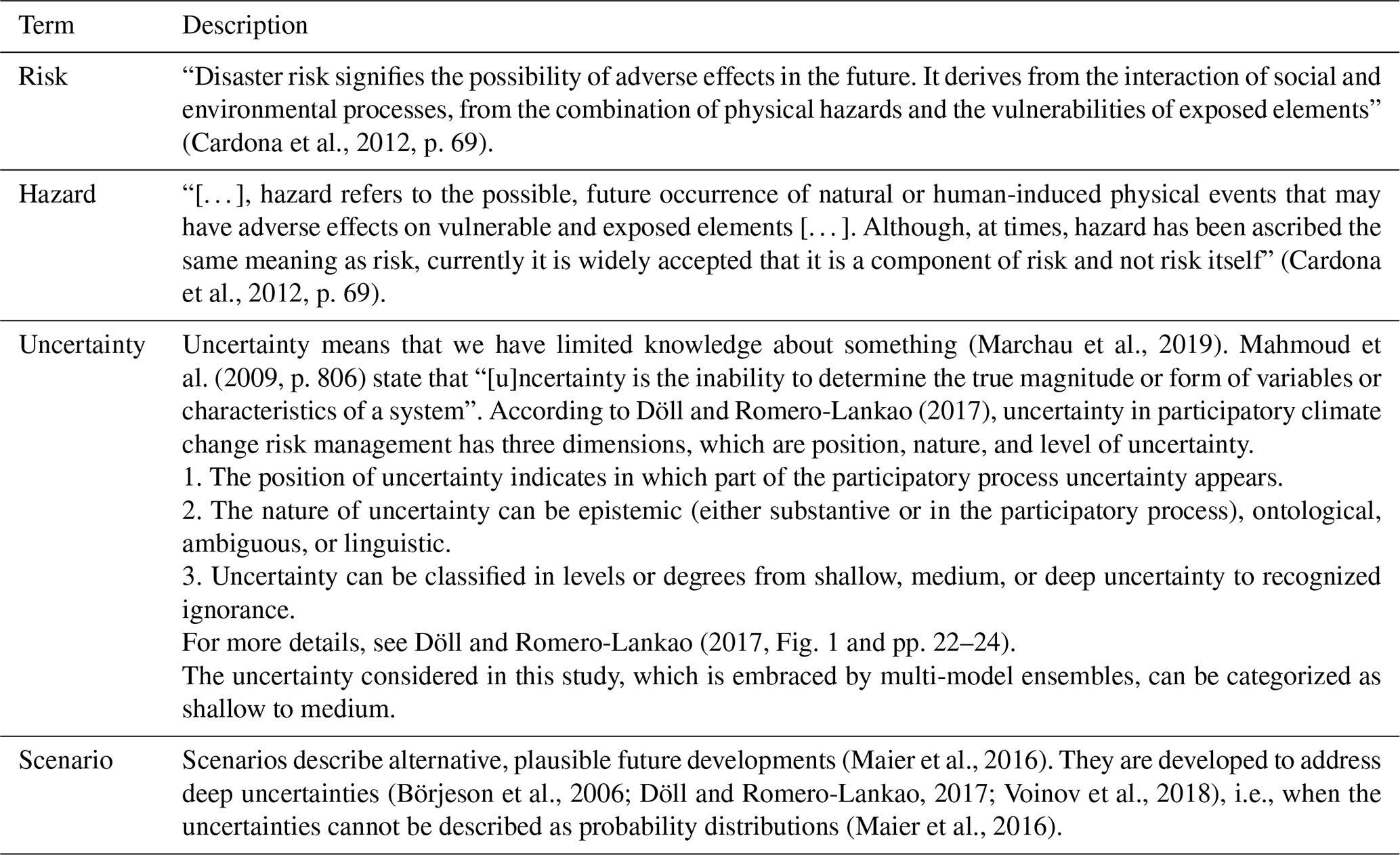
A4 Future period
The “far future around 2084” had to be shifted by 1 year compared to Hübener et al. (2017) due to the ISIMIP2b data only being available until 2099.
A5 Greenhouse gas emission scenarios
Scenario RCP 2.6 describes a pathway with strong mitigation measures resulting in global warming that likely will not exceed 2 °C until the end of the 21st century (compared to the “pre-industrial” period 1850–1900) and that therefore meets the goal of the Paris Agreement (Collins et al., 2013). Under RCP 8.5, high emissions of greenhouse gases are assumed, leading to global warming of approximately 4 °C until the end of the 21st century (Collins et al., 2013). The intermediate RCPs, RCP 4.5 and RCP 6.0, which are available in ISIMIP2b, were not used in this study to not overwhelm the stakeholders; the chosen RCPs 2.6 and 8.5 are to show the range of outcomes of the best-case and the worst-case climate futures.
A6 Area-weighted averages
Four of the 0.5° grid cells of the global hydrological models overlie the whole study area of about 2433 km2, covering 506, 532, 829, and 566 km2 (Fig. S1 in the Supplement). We calculated area-weighted averages for the BRR area from the four grid cell values and only used this average in our hazard quantification as global hydrological models cannot reliably quantify differences between the four grid cells and thus subregions of the BRR.
A7 Interannual variability
The exceedance probabilities were calculated with the annual averages, as well as the seasonal averages of the summer and winter months. We did not analyze floods as GHMs are not suitable for simulating local floods. We assessed droughts only by considering the change in statistical low-flow values of total runoff (particularly relevant for stream ecosystems) and groundwater recharge for both annual and summer values (see above).
A8 Relative changes in long-term mean changes
We calculated the potential relative changes in both groundwater recharge and total runoff between the reference period and the two future 30-year periods – the “near future around 2035” and the “far future around 2084” (Sect. 3.1). As indicators of the hydrological hazard of climate change, the changes between the 30-year periods were computed as relative changes for each GCM–GHM combination individually. For the interannual variability, we calculated the relative changes between the values of the same rank in the future and the reference period, resulting in changes in exceedance probabilities.
A9 Interpretation of 30-year mean change
For the annual values (gray percentile boxes), around 50 % of the multi-model ensemble simulates a decrease and around 50 % simulates an increase in total runoff and groundwater recharge in both future periods. For the seasonal values of total runoff, around half of the multi-model ensemble also simulates a decrease and around half simulates an increase for the near future around 2035, while a slight majority of the models predict an increase in the summer and winter months for the far future around 2084 (suggesting decreases in spring and autumn).
Regarding seasonal changes in groundwater recharge, at least 70 % of the multi-model ensemble simulates an increase in groundwater recharge during the winter months in both future periods and under both emissions scenarios. In contrast, at least 70 % of the multi-model ensemble simulates a decrease in groundwater recharge during the summer months in the near future around 2035 and in the far future around 2084 under the emissions scenario RCP 8.5. In the near future around 2035, 10 % of the model ensemble simulates a decrease of more than 50 % in groundwater recharge in summer months, while 10 % of the model ensemble simulates an increase of more than 65 % in groundwater recharge in winter months. In the far future around 2084 under the emissions scenario RCP 8.5, 10 % of the model ensemble simulates a decrease of more than 60 % in the summer months and an increase of more than 100 % in the winter months. For summer months in the far future around 2084 under the emissions scenario RCP 2.6, the median change is close to zero, but 10 % of the model ensemble projects a decrease of more than 50 %.
A10 Interpretation of interannual change
We assessed the changes in total runoff and groundwater recharge for all months, as well as for only the winter and summer months of each year. In the case of RCP 2.6, around 50 % of the multi-model ensemble simulates a decrease and around 50 % simulates an increase in groundwater recharge in years with relatively high summer groundwater recharge (left side of the right diagram in Fig. 6). The ensemble median (solid green line) drops to the right, and potential changes in groundwater recharge in those years with a relatively low summer recharge (from the exceedance probability of 70 %) of P70 (upper, dashed green line) drop below 0 %. This means that 70 % of the multi-model ensemble simulates a decrease in groundwater recharge in the case of relatively dry summers. In the case of RCP 8.5, at least 70 % of the multi-model ensemble simulates a decrease in groundwater recharge in the far future around 2084 under the emissions scenario RCP 8.5 in most wet and dry years. The ensemble median decrease in groundwater recharge becomes larger from wet to dry years, and 10 % of the ensemble members project that the summer recharge in wet years (10 % exceedance probability) will decrease by at least 45 %, but summer recharge in dry years (90 % exceedance probability) will decrease by at least 90 %. However, this behavior needs to be interpreted carefully because relative changes are higher for the same absolute change (in mm) when absolute values are small (Betts et al., 2018).
The map in Fig. S1 in the Supplement was created with ArcMap 10.8.1, available with a license from Esri at https://www.esri.com/en-us/home (Esri, 2020). The data used for Figs. 1, 5, and 6 are from the ISIMIP project, following the ISIMIP2b simulation protocol (ISIMIP, 2019), and can be accessed at https://www.isimip.org (last access: 27 October 2022, Frieler et al., 2017). The data were processed and analyzed with Python (https://www.python.org/, Python Software Foundation, 2019) in the Python integrated development environment PyCharm (available with a license at https://www.jetbrains.com/pycharm/. JetBrains s.r.o., 2023). The script and an example data set to generate a comparative figure of uncertainty visualization formats for the same data (Fig. 1) were made freely available (https://doi.org/10.5281/zenodo.10400312, Müller, 2023). The evaluation of the first workshop was realized with the SoSci Survey (Leiner, 2019) and was shared with the stakeholders via http://www.soscisurvey.de (last access: 16 May 2024). The evaluation results of the first workshop in the climate change adaptation process, which are shown in Fig. 8, are freely available in Zenodo (https://doi.org/10.5281/zenodo.7431706, Müller and Czymai, 2022; Creative Commons Attribution 4.0 International). The evaluation of the in-person presentation was realized with printouts, and that of the online presentation was realized in the webinar software edudip (https://www.edudip.com/, edudip GmbH, 2023) and downloaded as a PDF file. The evaluation results shown in Figs. 8 and 9 were digitalized and analyzed with Python (https://www.python.org/, last access: 16 May 2024) in the Python integrated development environment PyCharm (available with a license at https://www.jetbrains.com/pycharm/, last access: 16 May 2024) and the color-vision-deficiency-friendly color schemes were derived from Crameri (2018, https://doi.org/10.5281/zenodo.1243862). Figures 2 and 4, as well as the slides shown in Figs. 3 and 7, were created in Microsoft PowerPoint, available with a license at https://www.microsoft.com/de-de/microsoft-365 (Microsoft Corporation, 2016).
The supplement related to this article is available online at: https://doi.org/10.5194/gc-7-121-2024-supplement.
LM conducted the conceptualization, analysis, methodology, visualization, and writing of the original paper. PD had the original idea for the paper, supported and supervised all steps, and reviewed the paper.
The contact author has declared that neither of the authors has any competing interests.
The evaluations were carried out based on voluntary participation and informed consent to publish the outcomes. The evaluation data were gathered and saved in an anonymous manner. For this, the stakeholders were asked to evaluate (among others) the communication format in an online evaluation at the end of the digital workshop 1, and they were informed before that the evaluation results may be published anonymously. In the in-person presentation outside of the participatory process, consent documents were collected from each participant regarding their voluntary participation and their agreement to publish the evaluation results anonymously. In the online presentation outside of the participatory process, the audience was asked to evaluate the communication formats in an online evaluation, and they were informed that the evaluation results may be published anonymously. The research conducted in this study is novel, representing the authors' perspectives, and does not involve any intent to cause harm to others.
Publisher’s note: Copernicus Publications remains neutral with regard to jurisdictional claims made in the text, published maps, institutional affiliations, or any other geographical representation in this paper. While Copernicus Publications makes every effort to include appropriate place names, the final responsibility lies with the authors.
This article is part of the special issue “Climate and ocean education and communication: practice, ethics, and urgency”. It is not associated with a conference.
We thank Birgit Blättel-Mink and Max Czymai, with whom we organized and conducted the workshops in the KlimaRhön project. We are grateful for the support of the three administrations of the UNESCO biosphere reserve Rhön, who were the key stakeholders of the KlimaRhön project, and thank all the stakeholders who participated in the workshops for their engagement in the discussions. Moreover, we would like to thank the ISIMIP project (http://www.isimip.org, last access: 15 May 2024) and Hannes Müller Schmied for providing the model data. We are very thankful for the thorough comments of the reviewer Usha Harris, an anonymous reviewer, and the editors who helped to improve the paper. We acknowledge the use of ChatGPT for generating sentence examples and translations of specific words, contributing to the linguistic comprehensibility of our work.
This research has been supported by the Hessian Agency for Nature Conservation, Environment and Geology (HLNUG) and its Centre on Climate Change and Adaptation (FZK) (https://www.hlnug.de/themen/klimawandel-und-anpassung, last access: 16 May 2024).
This paper was edited by Solmaz Mohadjer and Sebastian G. Mutz and reviewed by Usha Harris and Asimina Voskaki.
Arias, P. A., Bellouin, N., Coppola, E., Jones, R. G., Krinner, G., Marotzke, J., Naik, V., Palmer, M. D., Plattner, G.-K., Rogelj, J., Rojas, M., Sillmann, J., Storelvmo, T., Thorne, P. W., Trewin, B., Achuta Rao, K., Adhikary, B., Allan, R. P., Armour, K., Bala, G., Barimalala, R., Berger, S., Canadell, J. G., Cassou, C., Cherchi, A., Collins, W., Collins, W. D., Connors, S. L., Corti, S., Cruz, F., Dentener, F. J., Dereczynski, C., Di Luca, A., Diongue Niang, A., Doblas-Reyes, F. J., Dosio, A., Douville, H., Engelbrecht, F., Eyring, V., Fischer, E., Forster, P., Fox-Kemper, B., Fuglestvedt, J. S., Fyfe, J. C., Gillett, N. P., Goldfarb, L., Gorodetskaya, I., Gutierrez, J. M., Hamdi, R., Hawkins, E., Hewitt, H. T., Hope, P., Islam, A. S., Jones, C., Kaufman, D. S., Kopp, R. E., Kosaka, Y., Kossin, J., Krakovska, S., Lee, J.-Y., Li, J., Mauritsen, T., Maycock, T. K., Meinshausen, M., Min, S.-K., Monteiro, P. M. S., Ngo-Duc, T., Otto, F., Pinto, I., Pirani, A., Raghavan, K., Ranasinghe, R., Ruane, A. C., Ruiz, L., Sallée, J.-B., Samset, B. H., Sathyendranath, S., Seneviratne, S. I., Sörensson, A. A., Szopa, S., Takayabu, I., Tréguier, A.-M., van den Hurk, B., Vautard, R., von Schuckmann, K., Zaehle, S., Zhang, X., and Zickfeld, K.: Technical Summary, in: Climate Change 2021: The Physical Science Basis. Contribution of Working Group I to the Sixth Assessment Report of the Intergovernmental Panel on Climate Change, edited by: Masson-Delmotte, V., Zhai, P., Pirani, A., Connors, S. L., Péan, C., Berger, S., Caud, N., Chen, Y., Goldfarb, L., Gomis, M. I., Huang, M., Leitzell, K., Lonnoy, E., Matthews, J. B. R., Maycock, T. K., Waterfield, T., Yelekçi, O., Yu, R., and Zhou, B., Cambridge University Press, Cambridge, United Kingdom and New York, NY, USA, 33–144, https://doi.org/10.1017/9781009157896.002, 2021.
Bammer, G.: Disciplining interdisciplinarity: Integration and implementation sciences for researching complex real-world problems, ANU E Press, Canberra ACT, Australia, 472 pp., http://www.jstor.org/stable/10.2307/j.ctt2jbkj5 (last access: 16 May 2024), ISBN 9781922144287, 2013.
Becker, E.: Transformations of Social and Ecological Issues into Transdisciplinary Research, in: Knowledge for Sustainable Development: An Insight into the Encyclopedia of Life Support Systems, 3, UNESCO-EOLSS, 949–963, ISBN 0 9542989-0-X, 2002.
Börjeson, L., Höjer, M., Dreborg, K.-H., Ekvall, T., and Finnveden, G.: Scenario types and techniques: towards a user's guide, Futures, 38, 723–739, https://doi.org/10.1016/j.futures.2005.12.002, 2006.
Cardona, O. D., van Aalst, M. K., Birkmann, J., Fordham, M., McGregor, G., Perez, R., Pulwarty, R. S., Schipper, E. L. F., and Sinh, B. T.: Determinants of risk: exposure and vulnerability, in: Managing the Risks of Extreme Events and Disasters to Advance Climate Change Adaptation: Special Report of the Intergovernmental Panel on Climate Change, edited by: Field, C. B., Barros, V., Stocker, T. F., Qin, D., Dokken, D. J., Ebi, K. L., Mastrandrea, M. D., Mach, K. J., Plattner, G.-K., Allen, S. K., Tignor, M., and Midgley, P. M., Cambridge University Press, Cambridge, UK, and New York, NY, USA, 65–108, https://doi.org/10.1017/CBO9781139177245.005, 2012.
Carlsson-Kanyama, A., Dreborg, K. H., Moll, H., and Padovan, D.: Participative backcasting: A tool for involving stakeholders in local sustainability planning, Futures, 40, 34–46, https://doi.org/10.1016/j.futures.2007.06.001, 2008.
Cash, D., Clark, W. C., Alcock, F., Dickson, N. M., Eckley, N., and Jäger, J.: Salience, Credibility, Legitimacy and Boundaries: Linking Research, Assessment and Decision Making, John F. Kennedy School of Government, Harvard University, Faculty Research Working Papers Series, https://doi.org/10.2139/ssrn.372280, 2002.
Collins, M., Knutti, R., Arblaster, J., Dufresne, J.-L., Fichefet, T., Friedlingstein, P., Gao, X., Gutowski, W. J., Johns, T., Krinner, G., Shongwe, M., Tebaldi, C., Weaver, A. J., and Wehner, M.: Long-term Climate Change: Projections, Commitments and Irreversibility, in: Climate Change 2013: The Physical Science Basis, Contribution of Working Group I to the Fifth Assessment Report of the Intergovernmental Panel on Climate Change, edited by: Stocker, T. F., Qin, D., Plattner, G.-K., Tignor, M., Allen, S. K., Boschung, J., Nauels, A., Xia, Y., Bex, V. and Midgley, P. M., Cambridge University Press, Cambridge, UK, and New York, NY, USA, 1029–1136, https://doi.org/10.1017/CBO9781107415324.024, 2013.
Corner, A., Shaw, C., and Clarke, J.: Principles for effective communication and public engagement on climate change: A Handbook for IPCC authors, Climate Outreach, Oxford, https://doi.org/10.13140/RG.2.2.28717.38884, 2018.
Crameri, F.: Scientific colour maps, Zenodo [code], https://doi.org/10.5281/zenodo.1243862, 2018.
Crosbie, R. S., Pickett, T., Mpelasoka, F. S., Hodgson, G., Charles, S. P., and Barron, O. V.: An assessment of the climate change impacts on groundwater recharge at a continental scale using a probabilistic approach with an ensemble of GCMs, Climatic Change, 117, 41–53, https://doi.org/10.1007/s10584-012-0558-6, 2013.
Czymai, M.: Die Cultural Theory of Risk als Erweiterung des systemtheoretischen Konfliktanalyserahmens für transdisziplinäre Forschungsprojekte, Soziologie und Nachhaltigkeit – Beiträge zur sozial-ökologischen Transformationsforschung, 9, 64–83, https://doi.org/10.17879/sun-2023-4956, 2023.
Daniels, E., Bharwani, S., Swartling, A. G., Vulturius, G., and Brandon, K.: Refocusing the climate services lens: Introducing a framework for co-designing “transdisciplinary knowledge integration processes” to build climate resilience, Climate Services, 19, 100181, https://doi.org/10.1016/j.cliser.2020.100181, 2020.
Davie, J. C. S., Falloon, P. D., Kahana, R., Dankers, R., Betts, R., Portmann, F. T., Wisser, D., Clark, D. B., Ito, A., Masaki, Y., Nishina, K., Fekete, B., Tessler, Z., Wada, Y., Liu, X., Tang, Q., Hagemann, S., Stacke, T., Pavlick, R., Schaphoff, S., Gosling, S. N., Franssen, W., and Arnell, N.: Comparing projections of future changes in runoff from hydrological and biome models in ISI-MIP, Earth Syst. Dynam., 4, 359–374, https://doi.org/10.5194/esd-4-359-2013, 2013.
Döll, P. and Romero-Lankao, P.: How to embrace uncertainty in participatory climate change risk management – A roadmap, Earth's Future, 5, 18–36, https://doi.org/10.1002/2016EF000411, 2017.
Döll, P., Jiménez-Cisneros, B., Oki, T., Arnell, N., Benito, G., Cogley, J. G., Jiang, T., Kundzewicz, Z. W., Mwakalila, S., and Nishijima, A.: Integrating risks of climate change into water management, Hydrolog. Sci. J., 60, 4–13, https://doi.org/10.1080/02626667.2014.967250, 2015.
edudip GmbH: edudip, edudip GmbH [code], https://www.edudip.com/ (last access: 16 May 2024), 2023.
Ertl, G., Bug, J., Elbracht, J., Engel, N., and Herrmann, F.: Grundwasserneubildung von Niedersachsen und Bremen – Berechnungen mit dem Wasserhaushaltsmodell mGROWA18, GeoBerichte 36, Landesamt für Bergbau, Energie und Geologie, 2019.
Esri: ArcGIS Desktop (Version 10.8.1), Esri [code], https://www.esri.com/en-us/home (last access: 16 May 2024), 2020.
Frieler, K., Lange, S., Piontek, F., Reyer, C. P. O., Schewe, J., Warszawski, L., Zhao, F., Chini, L., Denvil, S., Emanuel, K., Geiger, T., Halladay, K., Hurtt, G., Mengel, M., Murakami, D., Ostberg, S., Popp, A., Riva, R., Stevanovic, M., Suzuki, T., Volkholz, J., Burke, E., Ciais, P., Ebi, K., Eddy, T. D., Elliott, J., Galbraith, E., Gosling, S. N., Hattermann, F., Hickler, T., Hinkel, J., Hof, C., Huber, V., Jägermeyr, J., Krysanova, V., Marcé, R., Müller Schmied, H., Mouratiadou, I., Pierson, D., Tittensor, D. P., Vautard, R., van Vliet, M., Biber, M. F., Betts, R. A., Bodirsky, B. L., Deryng, D., Frolking, S., Jones, C. D., Lotze, H. K., Lotze-Campen, H., Sahajpal, R., Thonicke, K., Tian, H., and Yamagata, Y.: Assessing the impacts of 1.5 °C global warming – simulation protocol of the Inter-Sectoral Impact Model Intercomparison Project (ISIMIP2b), Geosci. Model Dev., 10, 4321–4345, https://doi.org/10.5194/gmd-10-4321-2017, 2017.
Hintze, J. L. and Nelson, R. D.: Violin Plots: A Box Plot-Density Trace Synergism, Am. Stat., 52, 181–184, https://doi.org/10.1080/00031305.1998.10480559, 1998.
Hofmann, H., Wickham, H., and Kafadar, K.: Letter-Value Plots: Boxplots for Large Data, J. Comput. Graph. Stat., 26, 469–477, https://doi.org/10.1080/10618600.2017.1305277, 2017.
Höllermann, B. and Evers, M.: Perception and handling of uncertainties in water management – A study of practitioners' and scientists' perspectives on uncertainty in their daily decision-making, Environ. Sci. Policy, 71, 9–18, https://doi.org/10.1016/j.envsci.2017.02.003, 2017.
Höllermann, B. and Evers, M.: Coping with uncertainty in water management: Qualitative system analysis as a vehicle to visualize the plurality of practitioners' uncertainty handling routines, J. Environ. Manage., 235, 213–223, https://doi.org/10.1016/j.jenvman.2019.01.034, 2019.
Hübener, H., Bülow, K., Fooken, C., Früh, B., Hoffmann, P., Höpp, S., Keuler, K., Menz, C., Mohr, V., Radtke, K., Ramthun, H., Spekat, A., Steger, C., Toussaint, F., Warrach-Sagi, K., and Woldt, M.: ReKliEs-De Ergebnisbericht, Technical report, Hessisches Landesamt für Naturschutz, Umwelt und Geologie, https://doi.org/10.2312/WDCC/ReKliEsDe_Ergebnisbericht, 2017.
ISIMIP: ISIMIP2b Simulation Protocol, https://www.isimip.org/protocol/2b/ (last access: 26 October 2022), 2019.
Jack, C. D., Jones, R., Burgin, L., and Daron, J.: Climate risk narratives: An iterative reflective process for co-producing and integrating climate knowledge, Climate Risk Management, 29, 100239, https://doi.org/10.1016/j.crm.2020.100239, 2020.
JetBrains s.r.o.: PyCharm 2023.2.1 (Professional Edition), JetBrains s.r.o. [code], https://www.jetbrains.com/pycharm/ (last access: 16 May 2024), 2023.
Kloprogge, P., van der Sluijs, J., and Wardekker, A.: Uncertainty communication: issues and good practice, Copernicus Institute for Sustainable Development and Innovation, Utrecht, The Netherlands, ISBN 978-90-8672-026-2, 2007.
Kneier, F., Woltersdorf, L., Peiris, T. A., and Döll, P.: Participatory Bayesian Network modeling of climate change risks and adaptation regarding water supply: Integration of multi-model ensemble hazard estimates and local expert knowledge, Environ. Modell. Softw., 168, 105764, https://doi.org/10.1016/j.envsoft.2023.105764, 2023.
Kok, K. and van Vliet, M.: Using a participatory scenario development toolbox: added values and impact on quality of scenarios, J. Water Clim. Change, 2, 87–105, https://doi.org/10.2166/wcc.2011.032, 2011.
Krueger, T., Maynard, C., Carr, G., Bruns, A., Mueller, E. N., and Lane, S.: A transdisciplinary account of water research, Wiley Interdisciplinary Reviews: Water, 3, 369–389, https://doi.org/10.1002/wat2.1132, 2016.
Lange, A., Ebert, S., and Vetter, A.: Adaptation Requires Participation: Criteria and Factors for Successful Stakeholder Interactions in Local Climate Change Adaptation, in: Handbook of Climate Change Management, edited by: Leal Filho, W., Luetz, J., and Ayal, D., Springer, Cham, Switzerland, 1–30, https://doi.org/10.1007/978-3-030-22759-3_47-1, 2021.
Lange, S., Volkholz, J., Geiger, T., Zhao, F., Vega, I., Veldkamp, T., Reyer, C. P. O., Warszawski, L., Huber, V., Jägermeyr, J., Schewe, J., Bresch, D. N., Büchner, M., Chang, J., Ciais, P., Dury, M., Emanuel, K., Folberth, C., Gerten, D., Gosling, S. N., Grillakis, M., Hanasaki, N., Henrot, A.-J., Hickler, T., Honda, Y., Ito, A., Khabarov, N., Koutroulis, A., Liu, W., Müller, C., Nishina, K., Ostberg, S., Müller Schmied, H., Seneviratne, S. I., Stacke, T., Steinkamp, J., Thiery, W., Wada, Y., Willner, S., Yang, H., Yoshikawa, M., Yue, C., and Frieler, K.: Projecting Exposure to Extreme Climate Impact Events Across Six Event Categories and Three Spatial Scales, Earth's Future, 8, e2020EF001616, https://doi.org/10.1029/2020EF001616, 2020.
Leiner, D. J.: SoSci Survey (Version 3.1.06) [code], https://www.soscisurvey.de (last access: 16 May 2024), 2019.
Lemos, M. C., Kirchho, C. J., and Ramprasad, V.: Narrowing the climate information usability gap, Nat. Clim. Change, 2, 789–794, https://doi.org/10.1038/nclimate1614, 2012.
Lux, A. and Burkhart, S.: Transdisziplinarität in der Anpassungsforschung – Eine Dokumenten- und Literaturanalyse, Climate Change, 2, Umweltbundesamt, Dessau-Roßlau, Germany, ISSN 1862-4359, 2023.
Mahmoud, M., Liu, Y., Hartmann, H., Stewart, S., Wagener, T., Semmens, D., Stewart, R., Gupta, H., Dominguez, D., Dominguez, F., Hulse, D., Letcher, R., Rashleigh, B., Smith, C., Street, R., Ticehurst, J., Twery, M., van Delden, H., Waldick, R., White, D., and Winter, L.: A formal framework for scenario development in support of environmental decision-making, Environ. Modell. Softw., 24, 798–808, https://doi.org/10.1016/j.envsoft.2008.11.010, 2009.
Maier, H. R., Guillaume, J. H., van Delden, H., Riddell, G. A., Haasnoot, M., and Kwakkel, J. H.: An uncertain future, deep uncertainty, scenarios, robustness and adaptation: How do they fit together?, Environ. Modell. Softw., 81, 154–164, https://doi.org/10.1016/j.envsoft.2016.03.014, 2016.
Mankin, J. S., Lehner, F., Coats, S., and McKinnon, K. A.: The Value of Initial Condition Large Ensembles to Robust Adaptation Decision-Making, Earth's Future, 8, e2012EF001610, https://doi.org/10.1029/2020EF001610, 2020.
Marchau, V. A., Walker, W. E., Bloemen, P. J., and Popper, S. W. (Eds.): Decision Making under Deep Uncertainty: From Theory to Practice, Springer Nature, Cham, Switzerland, https://doi.org/10.1007/978-3-030-05252-2, 2019.
Mearns, L. O.: The drama of uncertainty, Climatic Change, 100, 77–85, https://doi.org/10.1007/s10584-010-9841-6, 2010.
Microsoft Corporation: Microsoft PowerPoint 2016, Microsoft Corporation [code], https://www.microsoft.com/de-de/microsoft-365 (last access: 16 May 2024), 2016.
Milly, P. C., Betancourt, J., Falkenmark, M., Hirsch, R. M., Kundzewicz, Z. W., Lettenmaier, D. P., and Stouffer, R. J.: Stationarity is dead: Whither water management?, Science, 319, 573–574, https://doi.org/10.1126/science.1151915, 2008.
Müller, L.: Comparison of uncertainty visualization formats for participatory climate change adaptation processes, Zenodo [code], https://doi.org/10.5281/zenodo.10400312, 2023.
Müller, L. and Czymai, M.: Evaluations of the workshops 1, 2 and 3 in the participatory process of the project KlimaRhön, Zenodo [data set], https://doi.org/10.5281/zenodo.7431706, 2022.
Parviainen, T., Goerlandt, F., Helle, I., Haapasaari, P., and Kuikka, S.: Implementing Bayesian networks for ISO 31000: 2018-based maritime oil spill risk management: State-of-art, implementation benefits and challenges, and future research directions, J. Environ. Manage., 278, 111520, https://doi.org/10.1016/j.jenvman.2020.111520, 2020.
Python Software Foundation: Python (Version 3.7.6), Python Software Foundation [code], https://www.python.org/ (last access: 16 May 2024), 2019.
Reinecke, R., Müller Schmied, H., Trautmann, T., Andersen, L. S., Burek, P., Flörke, M., Gosling, S. N., Grillakis, M., Hanasaki, N., Koutroulis, A., Pokhrel, Y., Thiery, W., Wada, Y., Yusuke, S., and Döll, P.: Uncertainty of simulated groundwater recharge at different global warming levels: a global-scale multi-model ensemble study, Hydrol. Earth Syst. Sci., 25, 787–810, https://doi.org/10.5194/hess-25-787-2021, 2021.
Riedel, T. and Weber, T. K.: The influence of global change on Europe's water cycle and groundwater recharge, Hydrogeol. J., 28, 1939–1959, https://doi.org/10.1007/s10040-020-02165-3, 2020.
Rosener, J. B.: User-Oriented Evaluation: A New Way to View Citizen Participation, J. Appl. Behav. Sci., 17, 583–596, 1981.
Schönthaler, K. and Andrian-Werburg, S. V.: Erster integrierter Umweltbericht für das länderübergreifende UNESCO-Biosphärenreservat Rhön (Langfassung), Bayerisches Staatsministerium für Umwelt, Gesundheit und Verbraucherschutz (BaySt-MUGV), Hessisches Ministerium für Umwelt, ländlichen Raum und Verbraucherschutz (HMULV), and Thüringer Ministerium für Landwirtschaft, Naturschutz und Umwelt (TMLNU), Germany, ISBN 978-3-00-024013-3m 2008.
Scrieciu, A., Pagano, A., Coletta, V. R., Fratino, U., and Giordano, R.: Bayesian Belief Networks for Integrating Scientific and Stakeholders' Knowledge to Support Nature-Based Solution Implementation, Front. Earth Sci., 9, 674618, https://doi.org/10.3389/feart.2021.674618, 2021.
Spiegelhalter, D., Pearson, M. and Short, I.: Visualizing Uncertainty About the Future, Science, 333, 1393–1400, https://doi.org/10.1126/science.1191181, 2011.
Strasser, U., Vilsmaier, U., Prettenhaler, F., Marke, T., Steiger, R., Damm, A., Hanzer, F., Wilcke, R. A. I., and Stötter, J.: Coupled component modelling for inter- and transdisciplinary climate change impact research: Dimensions of integration and examples of interface design, Environ. Modell. Softw., 60, 180–187, https://doi.org/10.1016/j.envsoft.2014.06.014, 2014.
Tabari, H., Hosseinzadehtalaei, P., Thiery, W., and Willems, P.: Amplified Drought and Flood Risk Under Future Socioeconomic and Climatic Change, Earth's Future, 9, e2021EF002295, https://doi.org/10.1029/2021EF002295, 2021.
Tukey, J. W.: Exploratory Data Analysis, Addison-Wesley series in behavioral science: Quantitative methods, Addison-Wesley, Reading, Massachusetts, ISBN 9780201076165, 1997.
van der Bles, A. M., van der Linden, S., Freeman, A. L. J., Mitchell, J., Galvao, A. B., Zaval, L., and Spiegelhalter, D. J.: Communicating uncertainty about facts, numbers and science, Roy. Soc. Open Sci., 6, 181870, https://doi.org/10.1098/rsos.181870, 2019.
van Vuuren, D. P., Edmonds, J., Kainuma, M., Riahi, K., Thomson, A., Hibbard, K., Hurtt, G. C., Kram, T., Krey, V., Lamarque, J.-F., Masui, T., Meinshausen, M., Nakicenovic, N., Smith, S. J., and Rose, S. K.: The representative concentration pathways: an overview, Climatic Change, 109, 5–31, https://doi.org/10.1007/s10584-011-0148-z, 2011.
Verweij, M., Douglas, M., Ellis, R., Engel, C., Hendriks, F., Lohmann, S., Ney, S., Rayner, S., and Thompson, M.: Clumsy solutions for a complex world: the case of climate change, Public Admin., 84, 817-843, https://doi.org/10.1111/j.1540-8159.2005.09566.x-i1, 2006.
Voinov, A., Jenni, K., Gray, S., Kolagani, N., Glynn, P. D., Bommel, P., Prell, C., Zellner, M., Paolisso, M., Jordan, R., Sterling, E. J., Schmitt Olabisi, L., Giabbanelli, P. J., Sun, Z., Le Page, C., Elsawah, S., BenDor, T. K., Hubacek, K., Laursen, B. K., Jetter, A., Basco-Carrera, L., Singer, A., Young, L., Brunacini, J., and Smajgl, A.: Tools and methods in participatory modeling: Selecting the right tool for the job, Environ. Modell. Softw., 109, 232–255, https://doi.org/10.1016/j.envsoft.2018.08.028, 2018.
Warszawski, L., Frieler, K., Huber, V., Piontek, F., Serdeczny, O., and Schewe, J.: The inter-sectoral impact model intercomparison project (ISI-MIP): project framework, P. Natl. Acad. Sci. USA, 111, 3228–3232, https://doi.org/10.1073/pnas.1312330110, 2014.
- Abstract
- Introduction
- Visualization methods to communicate uncertain impacts of climate change
- Quantifying and communicating the uncertainty of the climate-change-induced hydrological hazards
- Results
- Discussion
- Conclusions
- Appendix A: Definition of central terms
- Data availability
- Author contributions
- Competing interests
- Ethical statement
- Disclaimer
- Special issue statement
- Acknowledgements
- Financial support
- Review statement
- References
- Supplement