Novel index to comprehensively evaluate air cleanliness: the Clean aIr Index (CII)

Air quality on our planet has been changing in particular since the industrial revolution (1750s) because of anthropogenic emissions. It is becoming increasingly important to realize air cleanliness, since clean air is as valuable a resource as clean water. A global standard for quantifying the level of air cleanliness is swiftly required, and we defined a novel concept, namely the Clean aIr Index (CII). The CII is a simple index defined by the normalization of the amount of a set of individual air pollutants. A CII value of 1 indicates completely clean air (no air pollutants), and 0 indicates the presence of air pollutants that meet the numerical environmental criteria for the normalization. In this time, the air pollutants used in the CII were taken from the Air Quality Guidelines (AQG) set by the World Health Organization (WHO), namely O₃, particulate matters, NO₂, and SO₂. We chose Japan as a study area to evaluate CII because of the following reasons: (i) accurate validation data, as the in situ observation sites of the Atmospheric Environmental Regional Observation System (AEROS) provide highly accurate values of air pollutant amounts, and (ii) fixed numerical criteria from the Japanese Environmental Quality Standards (JEQS) as directed by the Ministry of the Environment (MOE) of Japan. We quantified air cleanliness in terms of the CII for the all 1896 municipalities in Japan and used data from Seoul and Beijing to evaluate Japanese air cleanliness. The amount of each air pollutant was calculated using a model that combined the Weather Research and Forecasting (WRF) and Community Multiscale Air Quality (CMAQ) models for 1 April 2014 to 31 March 2017. The CII values calculated by the WRF–CMAQ model and the AEROS measurements showed good agreement. The mean of the correlation coefficient for the CII values of 498 municipalities where the AEROS measurements operated was 0.66±0.05, which was higher than that of the Air Quality Index (AQI) of 0.57±0.06. The CII values averaged for the study period were 0.67, 0.52, and 0.24 in Tokyo, Seoul, and Beijing, respectively; thus, the air in Tokyo was 1.5 and 2.3 times cleaner, i.e., lower amounts of air pollutants, than the air in Seoul and Beijing, respectively. The average CII value for the all Japanese municipalities was 0.72 over the study period. The extremely clean air, CII ≈0.90, occurred in the southern remote islands of Tokyo and to the west of the Pacific coast, i.e., Kochi, Mie, and Wakayama prefectures during summer, with the transport of clean air from the ocean. We presented the top 100 clean air cities in Japan as one example of an application of CII in society. We confirmed that the CII enabled the quantitative evaluation of air cleanliness. The CII can be useful and valuable in various scenarios such as encouraging sightseeing and migration, investment and insurance business, and city planning. The CII is a simple and fair index that can be applied to all nations.

1 Introduction

Air is an essential component for all life on our planet. Air quality has been changing since the industrial revolution (1750s). According to the report from OECD (2016), air pollutant emissions are predicted to increase because of the projected increase in the energy demand, e.g., transportation and power generation using fossil fuels, especially in East Asia. This report also mentions that the global annual market costs are predicted to increase from 0.3 % (in 2015) to 1.0 % (in 2060) of the global gross domestic product (GDP) because of reduced labor productivity, increased health expenditures, and crop yield losses due to air pollution.

A global standard index for quantifying air cleanliness should be developed in the same way that the Global Drinking Water Quality Index (GDWQI) has been developed for water quality, as defined by UNEP (2007), since clean air is as valuable a resource as clean water. Such an index can be a useful communication tool to help with decision-making. The index should be understandable and/or informative, not only for scientific experts but also for laypeople, and should also be upgraded with scientific data.

Several indices exist for estimating air quality, e.g., the Air Quality Index (AQI) in the United States (US; US EPA, 2006) and the Air Quality Health Index in Canada (Stieb et al., 2008) and Hong Kong (Wong et al., 2013). The purpose of these indices is to estimate health risks due to air pollution exposure. These indices were developed based on epidemiological studies and were optimized for each country or local area. The most commonly used index is the US AQI (US EPA, 2006). The AQI ranges from 0 to 500 and is calculated based on the concentrations of the six air pollutants. In the calculation of the AQI, an individual AQI for all air pollutants is calculated for a given location on a given day, and the maximum of all individual AQIs is defined as the overall AQI. Hu et al. (2015) performed a comparison study of several indices for air quality, using the measurements in China, and showed that AQI underestimates the severity of the health risks associated with exposure to multipollutant air pollution because AQI does not appropriately represent the combined effects of exposure to multiple pollutants. An index for quantifying the air quality is still under development, and the global standard has not been established yet.

In this study, we propose a novel concept for an index to quantify air cleanliness, namely the Clean aIr Index (CII), in order to establish the global standard for quantifying air cleanliness. The purpose of CII is to comprehensively evaluate air cleanliness by normalizing the amounts of common air pollutants with numerical environmental criteria. Here, we selected surface O₃, particulate matter (PM), NO₂, and SO₂ from the Air Quality Guidelines (AQG) set by the World Health Organization (WHO; WHO, 2005). As a first approach, we chose Japan for evaluating the CII because of (i) the validation data, as the in situ observation sites of the Atmospheric Environmental Regional Observation System (AEROS) provide highly accurate air pollutant amounts, and (ii) the fixed numerical criteria, i.e., from the Japanese Environmental Quality Standards (JEQS) as given by the Ministry of the Environment (MOE) of Japan.

In this paper, Sect. 2 defines the CII. Section 3 describes the model for calculating the CII for all Japanese municipalities and validates the CII values by comparing them with those derived from AEROS measurements. In Sect. 4, air cleanliness in each municipality is quantified, and the area and season of high air cleanliness in Japan is identified using the CII.

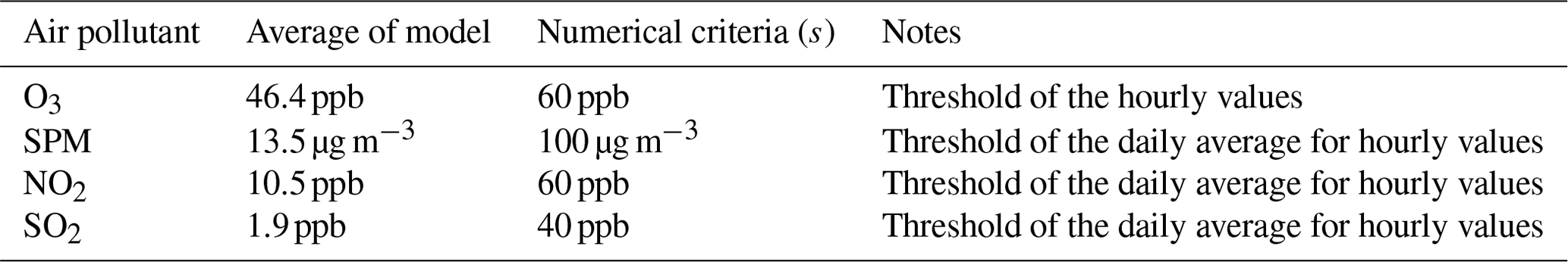
Table 1 Values of numerical criteria (s), O₃, suspended particulate matter (SPM), NO₂, and SO₂ used in this study. We used the criteria of the Japanese Environmental Quality Standards (JEQS) given by the Ministry of the Environment (MOE) of Japan. Averages of air pollutant amounts calculated by the model for all Japanese municipalities over the study period are shown. Note: ppb – parts per billion.

2 Clean aIr Index (CII)

The CII is a simple index defined by the normalization of each air pollutant amount. The definition of CII is given by the following:

$$\begin{array}{}\text{(1)}& \mathrm{CII}=f\left(x,s\right)=\mathrm{1}-{\displaystyle \frac{\mathrm{1}}{\mathrm{N}}}\sum _i^N{\displaystyle \frac{x\left[i\right]}{s\left[i\right]}},\end{array}$$

where x[i] is the amount of ith air pollutant, s[i] is the numerical criteria for the normalization of x[i], and N is the number of air pollutants considered in the CII. In this equation, a higher CII value indicates cleaner air, with a maximum of 1 indicating the absence of air pollutants. The CII value decreases as the amount of air pollutants increases, with a value of 0 indicating that the amount of air pollutants is equal to the numerical criteria and a negative value indicating that the amount of air pollutants is larger than the numerical criteria.

In this study, the air pollutants used in the CII are O₃, PM, NO₂, and SO₂, following the WHO AQG (WHO, 2005) as mentioned above, i.e., N=4. The field of this study is Japan; thus, we set the values of s according to the Japanese Environmental Quality Standards (JEQS), which are given by the Ministry of the Environment (MOE) of Japan (Table 1). The time length should be consistent between the x and s values when implementing the air pollutant amounts in the calculation of CII. In this case, the s value of O₃ is defined as a threshold for 1 h averages, and the values of the others are defined as 24 h averages. We employed the maximum of 1 h averages per day for O₃ and a daily mean for the other pollutants. We used the criterion for photochemical oxidants (O_x) in the JEQS as the s value for O₃ because more than 90 %–95 % of O_x is composed of O₃ (Akimoto, 2017). The CII can be used both globally and locally by defining the setting of s values. In the case of applying the CII to compare the air cleanliness globally, the numerical criteria should be given by the WHO AQG (WHO, 2005).

The selected air pollutants have been of importance for the last 5 decades in Japan and have been monitored by AEROS since 1970. Surface O₃, which is harmful to human health (e.g., Liu et al., 2013) and crop yields and quality (e.g., Feng et al., 2015; Miao et al., 2017), has been increasing in Japan since the 1980s in spite of the decreasing O₃ precursors such as NO_X and volatile organic compounds (VOCs; Akimoto et al., 2015). Nagashima et al. (2017) estimated that the source of surface O₃ is increasing, and approximately 50 % of the total increase was caused by transboundary pollution from China and Korea. We used the suspended particulate matter (SPM) for PM following the JEQS. NO₂ is a precursor of surface O₃ and is a harmful pollutant. It mostly originates from anthropogenic sources, especially fossil fuel combustion (e.g., power plants and vehicles). The environmental SO₂ level was severe in the 1970s in Japan. But the SO₂ concentration has been decreasing owing to the use of desulfurization technologies and low-sulfur fuel oil, and the JEQS for SO₂ was satisfied at most AEROS sites in 2012 (Wakamatsu et al., 2013).

3 Model simulation

A model simulation was performed to calculate the amounts of O₃, SPM, NO₂, and SO₂ for all Japanese municipalities (1896 in total; note that wards in megacities, such as Tokyo, Osaka, and Fukuoka were counted as independent municipalities). The AEROS measurement network does not cover the all municipalities; thus, we employed the model simulation. We combined two regional models, namely the Weather Research and Forecasting (WRF) model, to calculate meteorological fields (e.g., temperature, wind, and humidity), and the Community Multiscale Air Quality (CMAQ) model, to calculate air pollutant amounts using the WRF results as input parameters. Detailed descriptions about the WRF and CMAQ models are given in Sect. 3.1. The calculations were made from 22 March 2014 to 31 March 2017 and the outputs from 1 April 2014 to 31 March 2017, with intervals of every 1 h used for the analyses. We selected the simulation period with a unit of fiscal year (FY), starting on 1 April and ending on 31 March, because the AEROS measurement data set that we used to evaluate our simulation (Sect. 3.3) was archived with a unit of FY. The amount of SPM was simply assumed as being [SPM] = ([PM₁₀] + [PM_2.5]) ∕2 in this study.

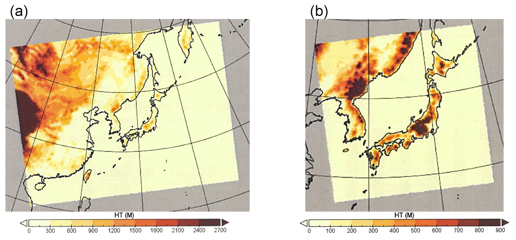
Figure 1 Ranges of (a) Domain 1 and (b) Domain 2 of the WRF–CMAQ models in this study. Color bars denote altitude.

3.1 WRF–CMAQ settings

We used the WRF model version 3.7 (Skamarock et al., 2008) to calculate the meteorological fields. We set two model domains, namely Domain 1, which covered East Asia with a horizontal grid resolution of 40 km and 157×123 grid points, and Domain 2, which covered mainland Japan with a horizontal grid resolution of 20 km and 123×123 grid points (see Fig. 1). The vertical layers consisted of 29 levels from the surface to 100 hPa. The initial and boundary conditions were obtained from the National Center for Environmental Prediction (NCEP) Final Operational Global Analysis (FNL; ds083.2) data (6 h; 1^∘ × 1^∘ resolution; NCEP FNL, 2000). In the model domain, 3D grid nudging for horizontal wind, temperature, and the water vapor mixing ratio and 2D grid nudging for sea surface temperature were performed every 6 h. Furthermore, we used the following parameterizations: the new Thompson scheme (Thompson et al., 2008) for microphysical parameterization, the Dudhia scheme (Dudhia, 1989) and rapid radiative transfer model (Mlawer et al., 1997) for short- and long-wave radiation processes, the Mellor–Yamada–Janjić scheme (Janjić, 1994) for planetary boundary layer parameterization, and the Betts–Yamada–Janjić scheme (Janjić, 1994) for cumulus parameterization.

The CMAQ model version 5.1 was used as a chemical transport model in this study. Byun and Schere (2006) provided an overview of the CMAQ model, and the updates and scientific evaluations of CMAQ version 5.1 are provided by Appel et al. (2017). For the gas-phase chemistry, the 2005 Carbon Bond (CB05) chemical mechanism, with the toluene update and additional chlorine chemistry (CB05TUCL, Yarwood et al., 2005; Whitten et al., 2010; Sarwar et al., 2012), was used. The core CB05 mechanism (Yarwood et al., 2005) has 51 chemical species and 156 reactions for the compounds and radicals of hydrogen, oxygen, carbon, nitrogen, and sulfur. Since then, the toluene update (Whitten et al., 2010) has improved the predictions of O₃ and NO_X productions and losses, dealing with 59 chemical species and 172 reactions in total. In addition, the implementation of chlorine chemistry (Sarwar et al., 2012) added seven chemical species and 25 reactions of chlorides, leading to increased O₃ and reduced nitrates. Regarding the photolysis of molecules, the photolysis rate preprocessor (JPROC) with 21 reactions (Roselle et al., 1999) has been implemented. Regarding the formations of aerosols, the combination of secondary organic aerosol (SOA) formations (Pye and Pouliot, 2012; Pye et al., 2013; Appel et al., 2017), ISORROPIA algorithms (Fountoukis and Nenes, 2007), and binary nucleation (VehkamäKi et al., 2002) has been implemented. A total of 45 kinds of aerosols components, including sulfate, ammonium, black carbon, organic carbon, and sea salt, have been considered in this model.

The molecules and aerosols were provided by the emissions (namely, anthropogenic, biogenic, and sea salt) from the surface or transport from the boundaries of domains and were transported by the wind fields calculated in the WRF model and the parameterizations of horizontal and/or vertical diffusions, dry deposition, and gravitational settling (see Byun and Schere, 2006; Appel et al., 2017). Anthropogenic emissions were defined using the MIX Asian emission inventory version 1.1, which included emissions from power, industry, residential, transportation, and agriculture sources (Li et al., 2017). This inventory of SO₂, NO_X, PM, VOCs, CO, and NH₃ for 2015 was estimated by correcting the 2010 data (2008 for NH₃) and was implemented into the CMAQ model. The corrections were made using the statistical secular changes in the annual total anthropogenic emissions of pollutants, and CO₂ (Crippa et al., 2019), population, amount of used chemical fertilizer, and NH₃ emissions by farm animals for each country were included in the model domains (Japan, China, South Korea, North Korea, Taiwan, Mongolia, Vietnam, and far-east Russia). Biogenic emissions of VOCs were provided by the Model of Emissions of Gases and Aerosols from Nature (MEGAN) version 2.10 (Guenther et al., 2012), using the meteorological fields calculated by the WRF model for 2016. Those implemented emission inventories did not include interannual changes. Volcanic emissions of SO₂ were ignored in our model simulation because of the following reasons. The SO₂ concentration values were averaged for 24 h to be consistent with the time length of the numerical criterion of JEQS; this procedure dilutes an increase in SO₂ due to volcanic eruption.

The CMAQ model used two model domains for which the regions were the same as those adopted in the WRF model (see Fig. 1) and had vertical coordinates of 22 layers; the thickness of the lowest layer was approximately 30 m. The initial and boundary conditions of air pollutants for Domain 1 were obtained from the Model for OZone And Related chemical Tracers (MOZART) version 4 (Emmons et al., 2010), and the boundary conditions for Domain 2 were the model outputs of Domain 1. The MOZART provided the distributions of more than 80 kinds of chemical species and aerosols for the inputs of our model calculations. The number of pollutants in each Japanese municipality were defined at the longitude and/or latitude of the municipal office, with the weighted average of the outputs at model grid points near the municipal office, using the following equation:

$$\begin{array}{}\text{(2)}& \stackrel{\mathrm{‾}}{A}={\displaystyle \frac{\mathrm{1}}{A_w}}\sum _{i=\mathrm{1}}^I{\displaystyle \frac{R^{\mathrm{2}}-d_i^{\mathrm{2}}}{R^{\mathrm{2}}+d_i^{\mathrm{2}}}}{A}_i,A_w=\sum _{i=\mathrm{1}}^I{\displaystyle \frac{R^{\mathrm{2}}-d_i^{\mathrm{2}}}{R^{\mathrm{2}}+d_i^{\mathrm{2}}}},\end{array}$$

where $\stackrel{\mathrm{‾}}{A}$ is the defined amount of a pollutant at the municipal office, I (=2 or 3, mostly) is the number of the model grid points of Domain 2 within $R=\sqrt{\mathrm{0.02}}$ degrees of the terrestrial central angle (approximately 16 km) from the office, and A_i and d_i are the simulated amounts of a pollutant and the distance from the office, respectively, at each model grid point. Note that Okinawa prefecture and Ogasawara-mura municipality in the Tokyo prefecture were outside Domain 2, and the number of pollutants at the municipalities in them were thus defined using the model outputs of Domain 1, with $R=\sqrt{\mathrm{0.08}}$ degrees (approximately 31 km) in Eq. (2). We also derived the number of pollutants in Seoul and Beijing for the comparisons with those inside Japan from the model outputs of Domain 1.

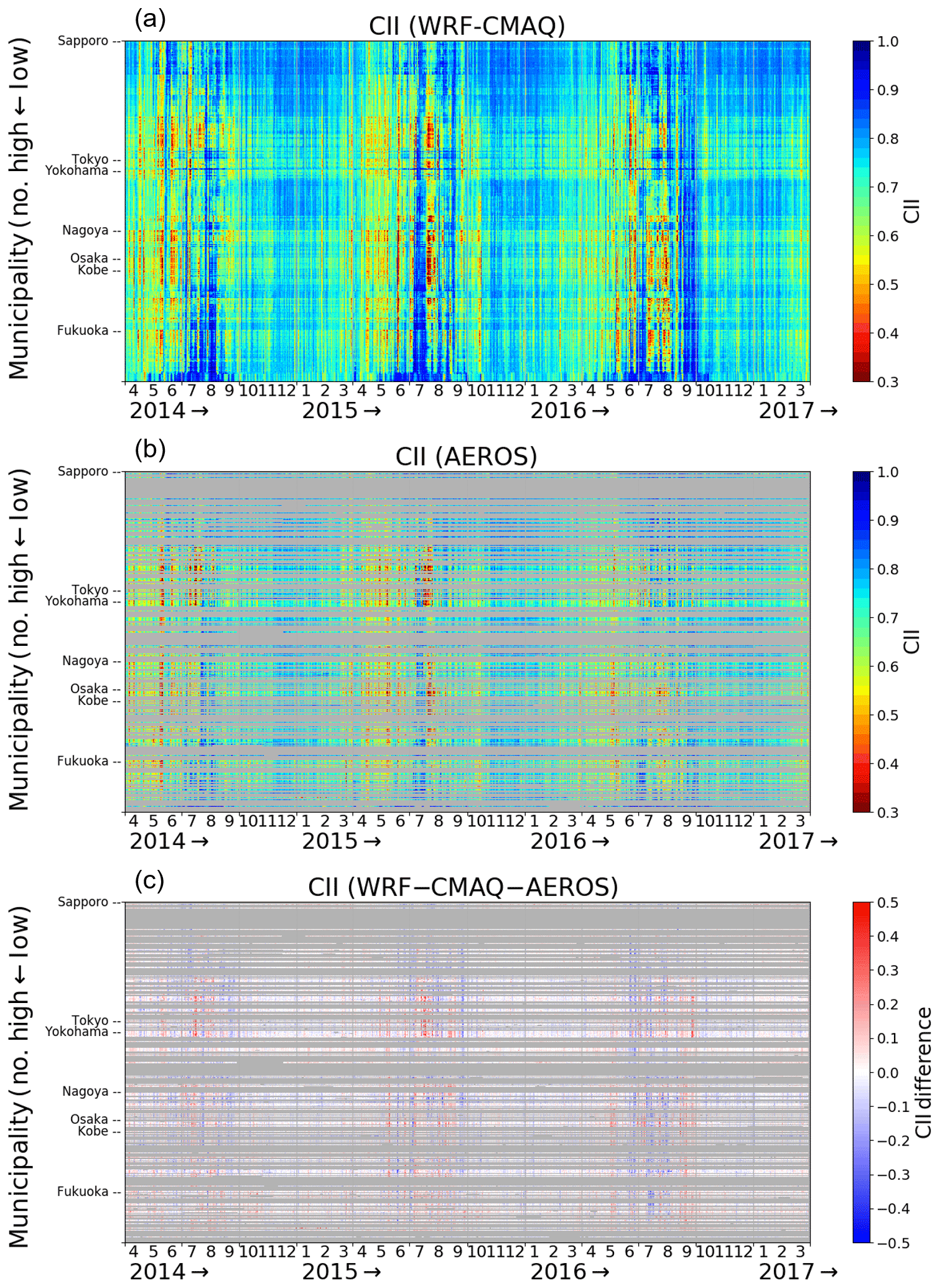
Figure 2 Spatiotemporal variation in CII values derived from (a) the WRF–CMAQ model, (b) the AEROS measurements, and (c) their difference (WRF–CMAQ–AEROS). The horizontal and vertical axes correspond to the date of the study period and Japanese municipal number, respectively. The municipalities where the AEROS observation covered less than 20 % of days in the study period are shaded in gray.

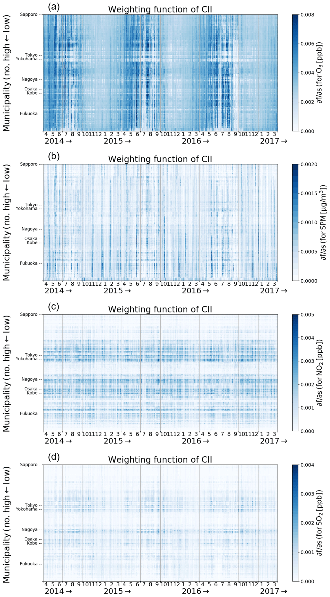
Figure 3 Spatiotemporal variation of the weighting function for the numerical criteria, K_s, for (a) O₃, (b) SPM, (c) NO₂, and (d) SO₂ derived from the WRF–CMAQ model. The color scaling is optimized for each panel.

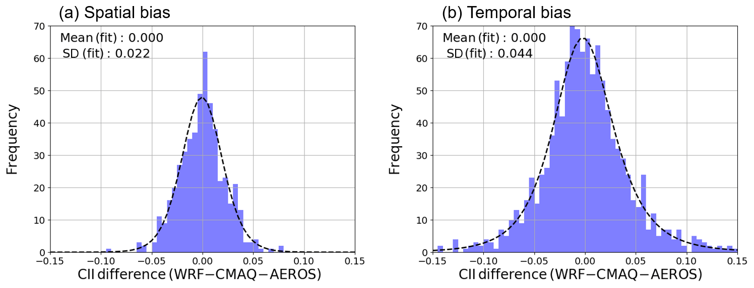
Figure 4 Histogram of the CII difference between the WRF–CMAQ model and the AEROS measurements. (a) The CII mean values of all days in the study period are compared for each municipality. (b) The CII mean values of all Japanese municipalities are compared for each day. The dashed line represents the fitting of the histogram of the CII difference by the Johnson SU function. The mean and standard deviation (1σ) values of the fitting function are shown in the upper left of each panel.

3.2 Spatiotemporal variation of CII

The spatiotemporal variations of CII based on the WRF–CMAQ model are shown in Fig. 2a. The horizontal and vertical axes correspond to the date and municipal number, respectively. The lower municipal number corresponds approximately to the municipalities in northeastern Japan, and vice versa, and the major cites in Japan are shown on the vertical axis. The CII value clearly depended on both area and season. The CII value tended to be higher in summer because of the transportation of unpolluted air masses from the Pacific Ocean. In August 2014, July 2015, and September 2016, the CII values of almost all municipalities were higher than 0.9 for a few weeks. However, the local CII values decreased to below 0.5 over a short period in summer because of local air pollutant emissions and the enhancement due to photochemical reactions induced by strong UV sunlight. The CII value was moderate (0.7–0.8) and stable from November to February over Japan but gradually decreased from February to May or June because polluted air was transported from East Asia (e.g., Park et al., 2014) and the sunlight strengthened.

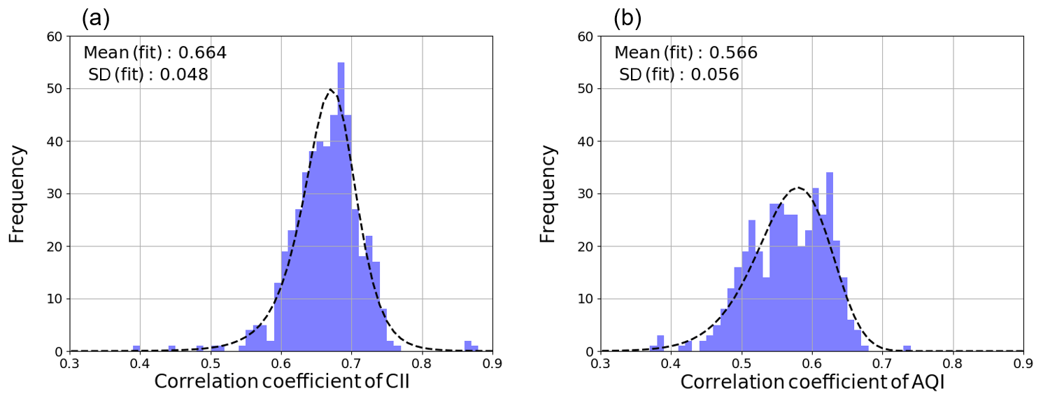
Figure 5 Histogram of the correlation coefficient (r) of the municipal mean of daily (a) CII and (b) AQI values for the study period between the WRF–CMAQ model and the AEROS measurements. The dashed line represents fitting of the histogram to the CII difference by the Johnson SU function. The mean and standard deviation (1σ) values of the fitting function are shown in the upper left of each panel.

These spatiotemporal features were reproduced by the AEROS measurements. Figure 2b and c show the time series variations in the daily CII value derived from the AEROS measurements and the difference (WRF–CMAQ–AEROS), respectively. AEROS is operated by the MOE of Japan and had 1901 observation sites for monitoring air pollutants in FY 2016. The AEROS data were obtained from the atmospheric environment database of the National Institute for Environmental Studies (i.e., the Kankyosuchi database in Japan). We used the AEROS observation sites that cover more than 80 % of the days in the study period, and a total of 498 of 1896 municipalities were covered by the AEROS measurements. The AEROS measurement results were averaged for all observation sites in each municipality in cases where there were several observation sites in one municipality. In this comparison, the AEROS O_x data were compared to the WRF–CMAQ O₃ data because the composition ratio was larger than 90 %–95 % O₃ in O_x (Akimoto, 2017).

The CII value depends not only on the amount of O₃, SPM, NO₂, and SO₂ (x), but also on the numerical criteria (s); see Eq. (1). A partial differentiation analysis was performed to determine the sensitivities of the s values of O₃, SPM, NO₂, and SO₂ to the CII. Figure 3 shows the weighting function for the numerical criteria (K_s) given by the following:

$$\begin{array}{}\text{(3)}& K_{\mathrm{s}}\left[i\right]={\displaystyle \frac{\partial f(x,s)}{\partial s\left[i\right]}}={\displaystyle \frac{\mathrm{1}}{N}}{\displaystyle \frac{x\left[i\right]}{s[i{]}^{\mathrm{2}}}}.\end{array}$$

As shown in Eq. (3), K_s positively correlates with x, and the CII value monotonically increases with increasing s. The temporal variation in CII primarily corresponded with the variation in O₃. The average K_s for O₃ was the highest among the species used to calculate the CII in this study because the x∕s value of O₃ was higher than those of SPM, NO₂, and SO₂ (Table 1). The value of K_s for SPM in western Japan was higher than in eastern Japan during winter and spring because of the effect of transboundary pollution from East Asia (e.g., Park et al., 2014). The spatial distribution of CII corresponded to that of K_s for NO₂ and SO₂, which explicitly reflected local emission sources such as those from megacities and industrial areas. The typical lifetime of NO₂ is approximately a few hours (e.g., Kenagy et al., 2018), and the transport effect was therefore less for these species. We ignored SO₂ emissions from volcanic eruptions, and the SO₂ distribution consequently corresponded to industrial activities. The spatial distribution of O₃ was negatively correlated to that of NO₂, primarily because of the Reactions (R1)–(R3).

3.3 Evaluation of spatial and temporal bias

We discuss the spatial and temporal bias in our calculation to clarify the magnitude of significant differences in the CII value. We compared the CII mean of all days in the study period between WRF–CMAQ and AEROS for each municipality. The CII difference for each municipality is shown in Fig. 4a to investigate the spatial bias. The histogram of the CII difference showed an asymmetrical distribution; thus, we fitted the histogram by using the Johnson SU function, which is a probability distribution transformed from the normal distribution to cover the asymmetry of the sample distribution (Johnson, 1949). The mean and standard deviations (1σ) of the CII difference were 0.00 and 0.02, respectively. In a similar way, we compared the CII mean of all Japanese municipalities for each day during the study period to investigate the daily temporal bias. Figure 4b shows the histogram of the CII difference for each day. The mean and standard deviations (1σ) of the CII difference were 0.00 and 0.04, respectively. Hereafter, we averaged the CII values for at least 30 d to compare the CII value among municipalities and to reduce the temporal bias to less than 0.01 ($\approx \mathrm{0.04}/\sqrt{\mathrm{30}}$). Consequently, the difference in CII derived from the WRF–CMAQ larger than 0.02 was significant enough to be reproduced by AEROS by averaging 30 values.

3.4 Comparison of CII and AQI

In Sect. 3.4, we discuss the difference between CII and AQI as representatives of indices for evaluating the air quality. We compared the indices calculated from the WRF–CMAQ model and the AEROS measurements. The mean of the correlation coefficient (r) for the study period between WRF–CMAQ and AEROS was calculated for each municipality. Figure 5 shows the histogram of r for all municipalities for (Fig. 5a) CII and (Fig. 5b) AQI. The histogram was fitted by the Johnson SU function. The r of CII and AQI was 0.66±0.05 (1σ) and 0.57±0.06 (1σ), respectively, and the CII showed better agreement between WRF–CMAQ and AEROS than AQI.

This discrepancy between CII and AQI is explained by the difference in their definitions. In the definition of AQI, only the air pollutants that cause the largest health risks are taken into account, and the other air pollutants are ignored (US EPA, 2006). In the definition of CII, four air pollutants, namely O₃, SPM, NO₂, and SO₂, are averaged with normalization by their numerical criteria, as in Eq. (1). It was reported that the amount of the surface O₃ was overestimated by the CMAQ model (Akimoto et al., 2019). In this case, NO₂ is underestimated because of the following reactions:

$$\begin{array}{}\text{(R1)}& {\displaystyle }{\mathrm{NO}}_{\mathrm{2}}+h\mathit{\nu }\to \mathrm{NO}+\mathrm{O},\text{(R2)}& {\displaystyle }\mathrm{O}+{\mathrm{O}}_{\mathrm{2}}+M\to {\mathrm{O}}_{\mathrm{3}}+M,\text{(R3)}& {\displaystyle }\mathrm{NO}+{\mathrm{O}}_{\mathrm{3}}\to {\mathrm{NO}}_{\mathrm{2}}+{\mathrm{O}}_{\mathrm{2}},\end{array}$$

where M is a third body for the ozone formation reaction. This discrepancy is less for CII than for AQI because the amounts of air pollutants are averaged by being normalized by the numerical criteria.

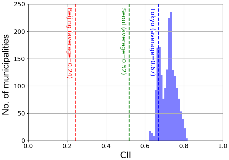
Figure 6 Histogram of average CII over the study period (FY 2014–2016) for each municipality in Japan. Red, green, and blue dashed lines represent the average CII of Beijing, Seoul, and Tokyo (23 wards), respectively.

Figure 7 Location of the Japanese municipalities focused on in this study. The municipal number is shown in parenthesis.

4 Visualization of air cleanliness in Japan

In Sect. 4, we discuss the area and season of high air cleanliness in Japan. Figure 6 shows the average CII over the study period (FY 2014–2016) for each Japanese municipality. The average CII of 85 % of the municipalities was higher than that of Tokyo (23 wards), and the average CII of all the municipalities was higher than those of Seoul and Beijing. Here the JEQS values were applied to the s values to calculate the CII values in Seoul and Beijing in order to directly compare them with those in the Japanese municipalities. The average and standard deviation (1σ) of CII was 0.67±0.10, 0.52±0.18, and 0.24±0.32 in Tokyo, Seoul, and Beijing, respectively. The value of 1 − CII monotonically increases as air pollutant amounts increase, and the air in Tokyo was 1.5 and 2.3 times cleaner, i.e., lower air pollutant amounts, than in Seoul and Beijing, respectively. The location of the municipalities discussed hereafter is shown in Fig. 7.

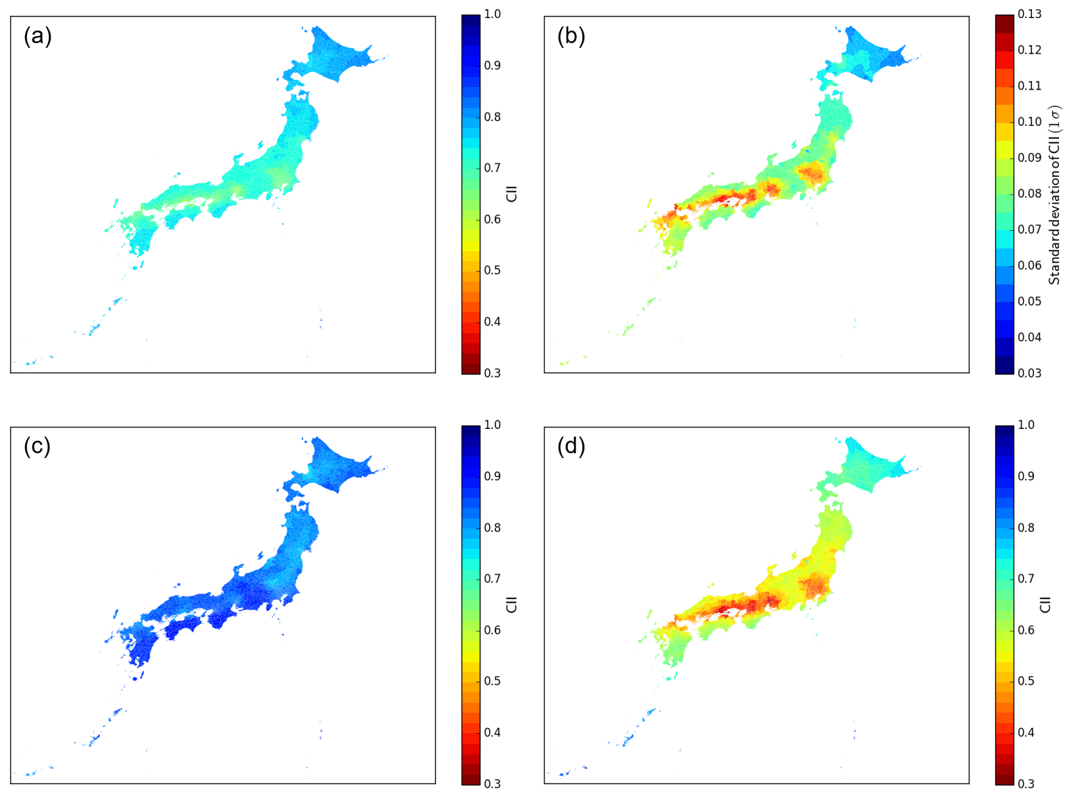
Figure 8 Spatial distributions of CII derived from the WRF–CMAQ model. (a) Mean over the study period (FY 2014–2016). (b) Same as (a) but for standard deviation (1σ). (c) Mean for 30 d of the highest CII average in all Japanese municipalities (10 d from each FY). (d) Same as (c) but for lowest CII average.

4.1 Area and season of high air cleanliness

We discuss the area and season of the highest air cleanliness over Japan using the CII in Sect. 4.1. First, the CII average over the study period, FY 2014–2016, in each municipality was compared in Fig. 8a. The CII averages in northern Japan were higher, and those in municipalities around megacities and industrial areas were lower than the average of all the municipalities, namely 0.72±0.04 (1σ). Table 2 shows the 10 municipalities with the highest average CII values which are located in eastern Hokkaido and the southern remote islands in Tokyo. The average CII was approximately 0.81 in these 10 municipalities, and the standard deviation (1σ) over the study period was lower than in other areas (see Fig. 8b), which means the CII remained high throughout the year. For example, the CII daily value in the Nemuro-shi municipality, where the 3-year CII average was the highest, was higher than the total municipal average of 0.72 % on 95 % of days over the study period.

Table 2 A total of 10 municipalities with the highest average CII value over the study period (FY 2014–2016). The municipal number is shown in parenthesis.

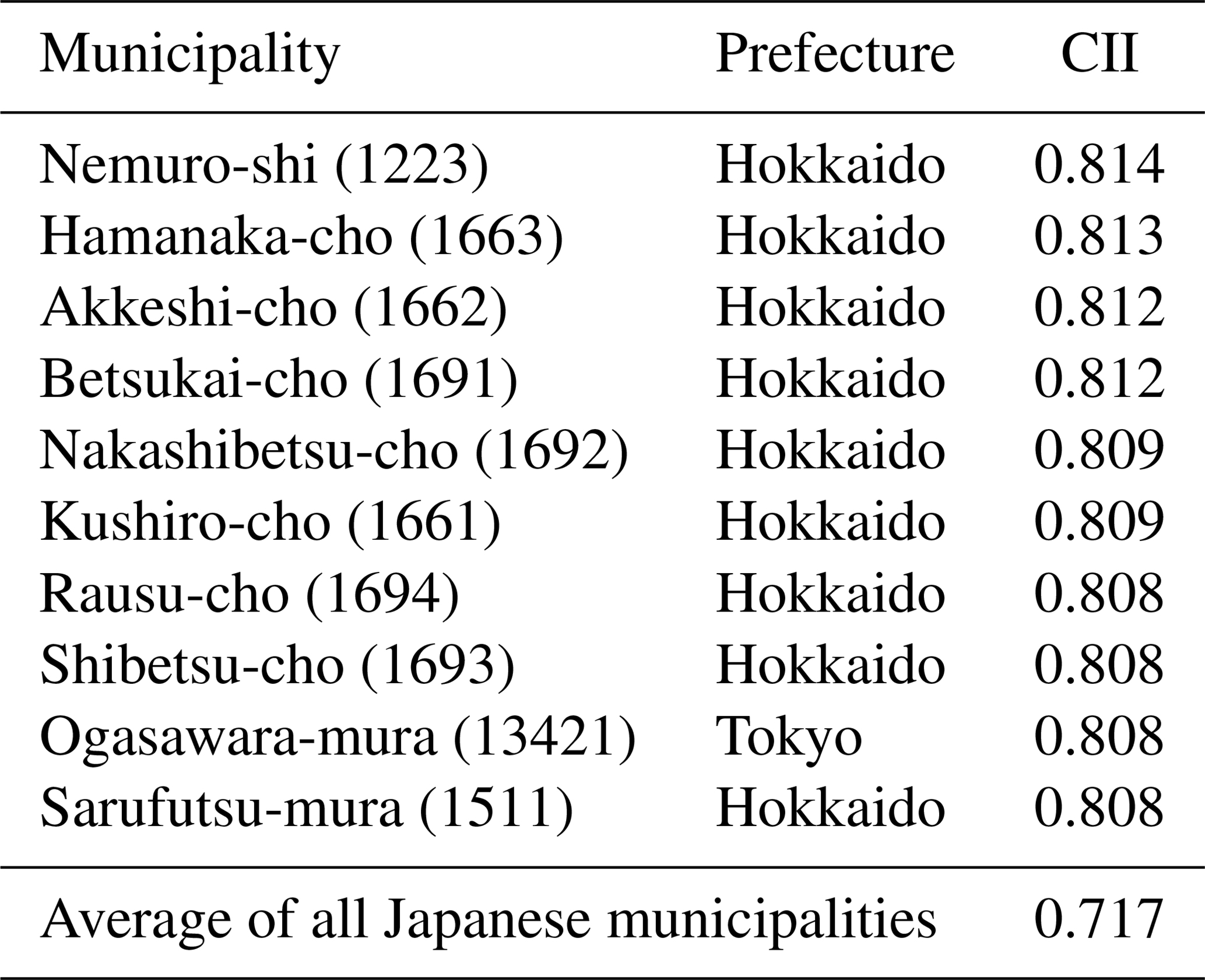
Table 3 Same as Table 2 but for the average CII for the 30 high-CII days.

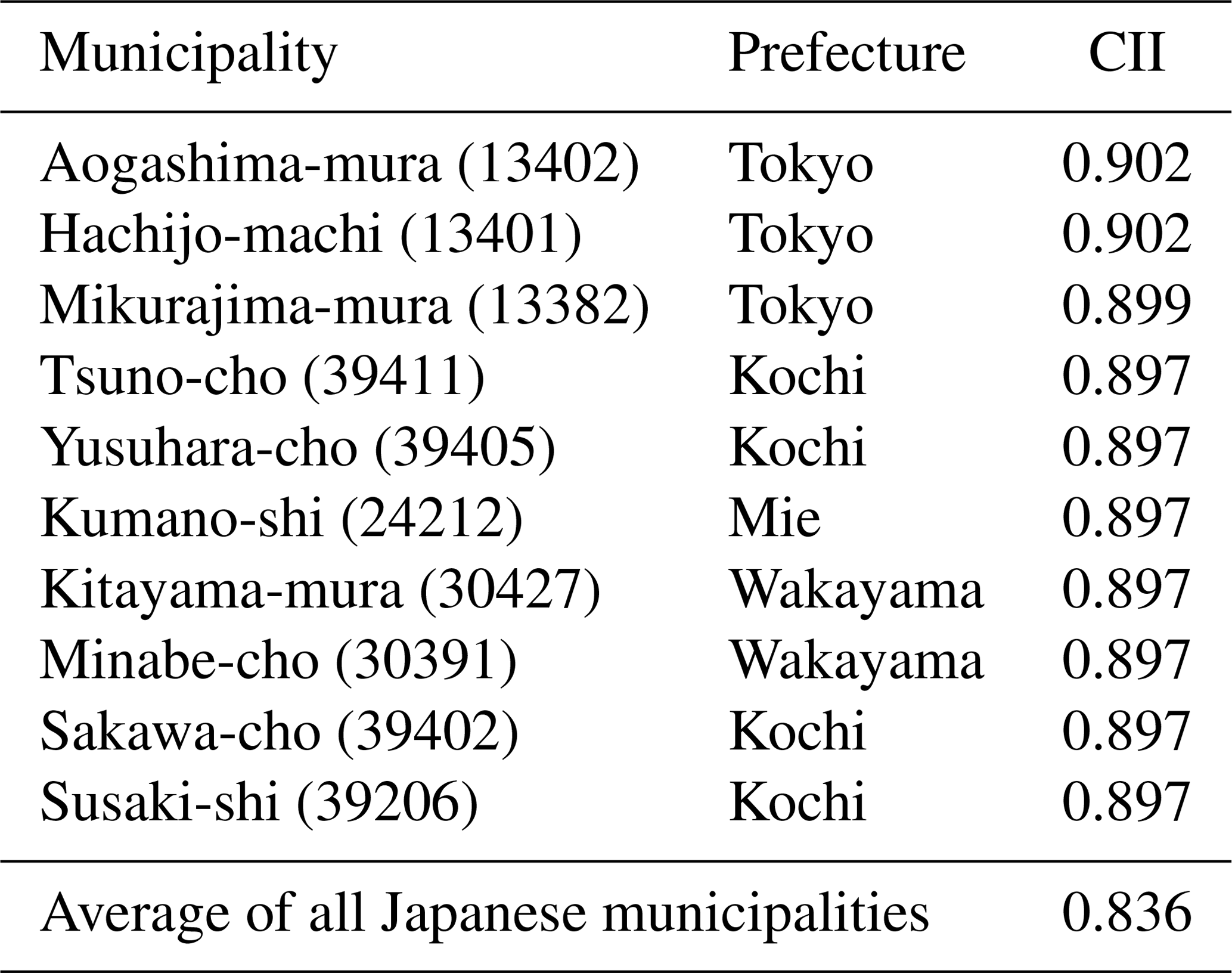
We discuss the CII distribution in the case of the high-CII average of all Japanese municipalities. We selected 10 d per year, a total of 30 d with the highest average CII values (09/07, 10/07, 09/08, 10/08, 15/08, 16/08, 18/08, 05/10, 06/12, and 12/01 in FY 2014; 09/07, 13/07, 16/07–19/07, 22/07, 17/08, 09/09, and 10/09 in FY 2015; and 09/07, 07/09, 12/09–14/09, 19/09, 20/09, 25/09, 27/09, and 28/09 in FY 2016). The 30 d CII values were averaged to discuss the CII distribution with the same order precision of 0.02 as the AEROS measurements (see Sect. 3.3). Almost all of these 30 d were in summer when unpolluted air was transported from the Pacific Ocean. The average CII values on these 30 d for each municipality are displayed in Fig. 8c, and Table 3 shows the 10 municipalities with the highest average CII values on these days. These 10 municipalities are located in the southern remote islands of Tokyo and the western Pacific coast area, i.e., the Kochi, Mie, and Wakayama prefectures. The average CII of the Aogashima-mura municipality in southern remote islands of the Tokyo prefecture was the highest. The average CII of these 10 municipalities was approximately 0.90, which was 0.06 on the CII scale, higher than all of the Japanese municipalities on high-CII days (0.84). Therefore, the highest CII value occurred on the Pacific coast during summer with low local pollution conditions.

Table 4 Same as Table 2 but for the average CII for the 30 low-CII days.

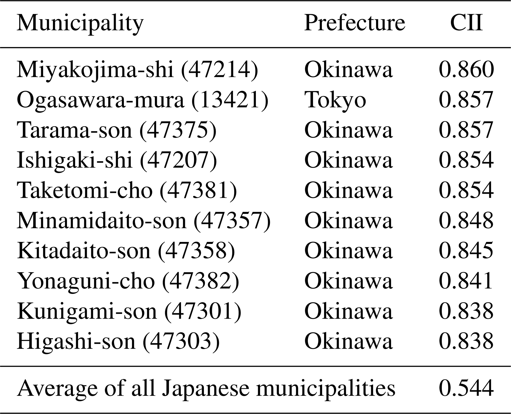
Table 5 A list of the top 100 clean air cities in Japan. The municipal number is shown in parenthesis.

Similar to the high-CII case, 30 d with the lowest CII average of all Japanese municipalities were selected (26/04, 29/05–02/06, 15/06, 16/06, 12/07, and 15/07 in FY 2014; 27/04, 13/05, 22/05, 27/05, 12/06, 13/06, 15/06, 31/07, 01/08, and 02/08 in FY 2015; and 27/05, 28/05, 31/05, 10/06, 17/06, 18/06, 26/06, 27/06, 11/08, and 01/09 in FY 2016). The averages of the CII values on these 30 low-CII days for each municipality are displayed in Fig. 8d, and Table 4 shows the 10 municipalities with the highest average CII values on these days. These 10 municipalities are located in the southern remote islands, such as Miyakojima-shi in the Okinawa prefecture and Ogasawara-mura in the Tokyo prefecture. The average CII in these municipalities was 0.84–0.86, which was approximately 0.30–0.32 on the CII scale, higher than that of all municipalities on low-CII days (0.54). The selected 30 d occurred especially at the end of spring and the beginning of summer. Generally, the transboundary pollution effect is large in the cold season, and heavy local pollution occurs in summer because of photochemical reactions induced by strong sunlight (e.g., Nagashima et al., 2010). These pollution effects are less pronounced in the remote islands; thus, the CII maintained higher values.

We selected the top 100 clean air cities in Japan as one example of CII use in society with the following method. The average of the 30 highest daily CII values in the study period was calculated for each municipality. The 30 d were selected for each municipality, not as in the case of Fig. 8c and d. Table 5 shows the 100 municipalities with the highest average CII values. The municipalities in the remote islands of Tokyo around western Japan, especially around the Pacific coast and Okinawa prefectures, were selected.

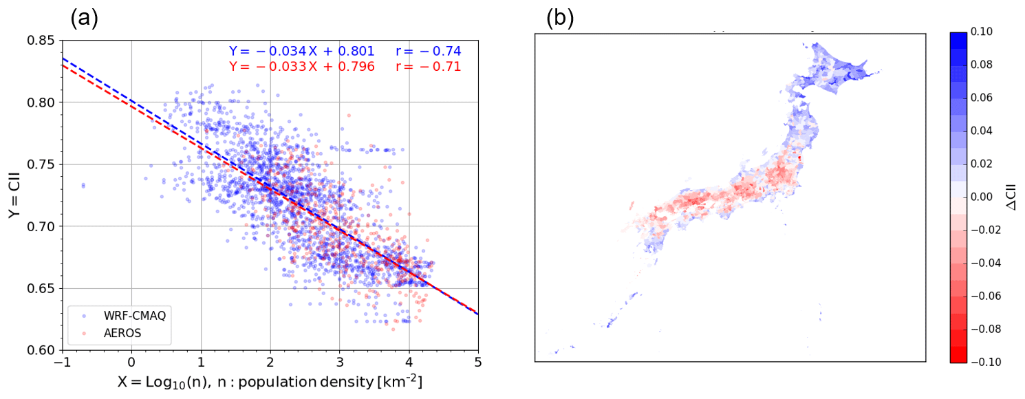
Figure 9 (a) Comparison of CII and population density (n) in each Japanese municipality. The dashed line shows the linear regression of CII with log₁₀(n). The correlation coefficient (r) between CII values and log₁₀(n) is also shown in the upper corner. The blue and red coloring shows the WRF–CMAQ and AEROS results, respectively. (b) Distribution of differences in CII from the linear regression (ΔCII) for the WRF–CMAQ model.

4.2 Air cleanliness and human activities

Industrial activities, particularly fossil fuel combustion such as vehicles and power plants, are major sources of air pollutants, and air cleanliness is strongly related to human activity. In Sect. 4.2, we discuss the municipalities in Japan with respect to not only air cleanliness but also human activity. We group them into the following four categories: (1) clean air with high human activity, (2) clean air with low human activity, (3) dirty air with high human activity, and (4) dirty air with low human activity. In this study, the common logarithm of population density (n), log₁₀(n), was employed to quantify human activities following, e.g., Kerr and Currie (1995). The n data were obtained from the 2015 Japanese national census (NSTAC, 2016). Figure 9a shows the scatterplot of log₁₀(n) and the average CII for the study period as derived from the WRF–CMAQ model and the AEROS measurements for each municipality. A clear negative correlation between log₁₀(n) and the CII was observed, and the r values were −0.74 and −0.71 for WRF–CMAQ and AEROS, respectively. This negative correlation was formulated by the linear regression with the objective variable of CII and the explanatory variable of log₁₀(n), as shown by the dashed lines in Fig. 9a.

$$\begin{array}{}\text{(R4)}& \text{Approximated CII}=a\times {\log }_{\mathrm{10}}\left(n\right)+b.\end{array}$$

The parameters of a and b were estimated to be $-\mathrm{0.034}\pm \mathrm{0.001}$ and 0.801±0.002 for WRF–CMAQ and $-\mathrm{0.033}\pm \mathrm{0.001}$ and 0.796±0.005 for AEROS, respectively. The negative correlation between log₁₀(n) and the CII value derived from WRF–CMAQ was reproduced by AEROS, and the parameters of a and b agreed within their errors.

The CII value showed a negative correlation with human activity; thus, the municipalities in groups 2 and 3 are in a normal situation. The municipalities in group 1 are an ideal case because such municipalities are expected to be industrially advanced and successful in maintaining a clean air environment. There are some issues in the municipalities in group 4 because such municipalities cannot have clean air in spite of their smaller population. It might indicate that there are large air pollution sources, such as large power plants, or air pollutants are transported from outside the region. The degree of this categorizing is quantified by the difference between the CII and the linear regression line, as per Eq. (R4), (ΔCII) as follows.

$$\begin{array}{}\text{(R5)}& \mathrm{\Delta }\text{CII}=\text{CII}-\text{Approximated CII}.\end{array}$$

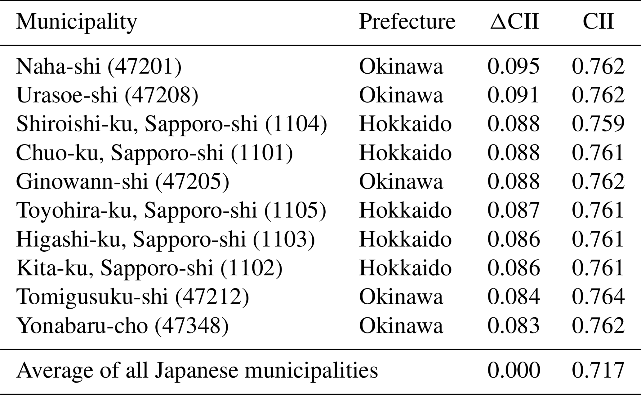
The positive ΔCII value means that the municipality is categorized in group 1, and the negative ΔCII value is group 4. The distribution of ΔCII in the average for the study period is shown in Fig. 9b, and Table 6 shows the 10 municipalities with the highest average ΔCII values. All of these municipalities were in the Hokkaido and Okinawa prefectures. The higher ΔCII values were observed in northeastern Japan and the coastal area. There are many industrial areas in western Japan (Li et al., 2017), which might be one reason for the lower ΔCII values. A combination of CII and ΔCII could be a useful way of evaluating air cleanliness in municipalities.

Table 6 A total of 10 municipalities with the highest average ΔCII value over the study period (FY 2014–2016). The municipal number is shown in parenthesis.

5 Conclusions

We defined a novel concept of indexing to quantify air cleanliness, namely CII. This index comprehensively evaluates the level of air cleanliness by normalizing the amounts of common air pollutants. A CII value of 1 indicates the absence of air pollutants, and 0 indicates that the amounts of air pollutants are the same as the normalization numerical criteria.

A model simulation was performed to visualize the air cleanliness of all 1896 municipalities in Japan using CII. We used O₃, SPM, NO₂, and SO₂ in this study, and their numerical environmental criteria were taken from the JEQS set by the MOE of Japan. The amounts of these species were calculated via the model, combining the WRF model version 3.7 and CMAQ model version 5.1. The time period of the simulation was from 1 April 2014 to 31 March 2017, i.e., FY 2014–2016. The CII values near the surface derived from the model were evaluated by comparing them with those of the AEROS in situ observations that are operated by the MOE of Japan. A total of 498 municipalities were covered by the AEROS measurements. The difference in CII between WRF–CMAQ and AEROS was distributed between 0.00±0.02 and 0.00±0.04 for spatial and temporal bias, respectively. We concluded that the difference in CII, derived from the WRF–CMAQ as being larger than 0.02, was significant enough to be reproduced by AEROS by averaging 30 values to reduce the temporal bias to less than 0.01 ($\approx \mathrm{0.04}/\sqrt{\mathrm{30}}$). The difference between CII and AQI was also discussed. The mean correlation coefficient (r) for the study period between WRF–CMAQ and AEROS was calculated for each municipality. The r of CII and AQI was 0.66±0.05 (1σ) and 0.57±0.06 (1σ), respectively. The CII showed better agreement between WRF–CMAQ and AEROS than AQI because of the difference in definition between CII and AQI. The CII averages all normalized air pollutant amounts, but the AQI employs only the maximum of the individual pollutants, i.e., any effects from the other air pollutants are ignored. This CII concept for comprehensively evaluating multiple air pollutants could be an advantage in the quantification of air cleanliness.

Over the study period, FY 2014–2016, the average CII value of Tokyo (23 wards), Seoul, and Beijing was 0.67, 0.52, and 0.24, respectively. This means that the air in Tokyo was 1.5 and 2.3 times cleaner, i.e., fewer air pollutants, than in Seoul and Beijing, respectively. The CII value varied spatially and temporally, corresponding to variations in O₃, SPM, NO₂, and SO₂. The municipalities in the eastern Hokkaido prefecture had the highest CII average values of approximately 0.81, which was 0.09 on the CII scale, higher than the average value of all Japanese municipalities (0.72). The extremely clean air, with CII values of approximately 0.90, occurred in the southern remote islands of Tokyo and around the western Pacific coast, i.e., Kochi, Mie, and Wakayama prefectures during summer with the transport of unpolluted air from the ocean. The municipalities in the southern remote islands in the Okinawa and Tokyo prefectures maintained their high-CII values of 0.84–0.86, which was approximately 0.30–0.32, which was approximately 0.30–0.32 on the CII scale, higher than that of all municipalities on low-CII days (0.54). Furthermore, the list of the top 100 clean air cities in Japan was presented as one example of how CII could be used in society.

We quantified the air cleanliness in the municipalities with respect to human industrial activities using population density. A negative correlation between CII and the population density was observed by both the WRF–CMAQ model and the AEROS measurement. The CII was approximated by a linear function of the common logarithm of population density. The differences in CII from this approximation line (ΔCII) indicate that the CII is weighted by human activity. The municipalities with positive ΔCII values are expected to maintain clean air and to be industrially advanced. Those with negative ΔCII values are expected to have certain issues, such as large air pollution sources and air pollutants being transported from outside. A combination of the CII and ΔCII could be a useful way of evaluating air cleanliness in a municipality.

The CII can be used in various scenarios, such as encouraging sightseeing and migration, investment and insurance business, and city planning. The CII can be used for an advertisement of clean air for local governments in order to promote sightseeing and migration. The CII is also effective for measuring the potential of local brands and tourism resources. Private companies can be expected to use CII for environmental, social, and governance (ESG) investments. If the CII were associated with life expectancy, the CII could be applied to insurance business, especially in Asian regions where urban air pollution is a serious problem. City planning is also a possible use of CII because air cleanliness is related to urban form (e.g., McCarty and Kaza, 2015). As mentioned above, the CII has the potential to be applied to policy and businesses in cities and countries around the world.